$2,620,670.84 bought thirty reinforcement-learning steps. Not thirty prompts, not thirty attempts at fixing a repository: thirty updates fed by 752,640 trained sequences, with agents, graders, sandboxes and a distributed training system doing the work between them. Xiaomi’s public MiMo-V2.6 run log leaves that bill visible. It also leaves visible the restarts. I find the second disclosure at least as useful as the first.
The argument of this article is that agentic RL is an exercise in protecting the meaning of a training signal across a messy software system. Better optimization matters. So do the supposedly peripheral details: which tokens were actually generated, whether a verifier was reachable, whether an agent found tomorrow’s answer in yesterday’s Git history, whether a screenshot exists on the machine doing the grading. MiMo’s report and public code make those connections unusually concrete without giving us enough evidence to call the whole production system reproduced.
There are two releases to understand, plus a distinction inside the software. Xiaomi describes large Pro and Flash production runs. It also publishes smaller, domain-specific recipes around a distilled 9B model. The framework contains capabilities beyond what those recipes enable. Confusing these levels produces an impressive headline and a bad technical explanation. Keeping them separate produces something much more useful: a picture of how the machinery works, what can be inspected, and what still requires an experiment.
The technical report calls its central training approach “You Only RL Once”: one large mixed-task RL run rather than a procession of separate domain RL stages. That name does not mean pretraining vanished, that supervised fine-tuning became unnecessary, or that no distillation followed RL. All three remain in the reported pipeline. Nor does the release turn a 9B training script into a trillion-parameter production deployment. The small lane is valuable on its own terms.
My earlier MiMo v2.5 Pro coding test concerned using a model. This piece concerns the system that shapes one. It draws on a completed report digest, saved public telemetry, and a multi-worker source review with a later correction pass. It does not claim every file was read. No training, evaluation, package installation, cluster preflight, weight download or container launch was performed for this article. The runbook below is documentary: it explains the inspected launch contracts, not a successful reproduction we secretly performed offstage.
That boundary is not a disclaimer to tuck beneath the credits. It changes how almost every number should be read. A reported ablation is evidence from Xiaomi, not our measurement. A function in a public repository proves that the function exists, not that a particular launch path calls it. A default in YAML establishes an intention until the consuming code has been traced. And a public dashboard can disagree with the tidy range in a report without either disagreement being solved by more enthusiastic prose.
A release with three different kinds of truth
The production layer begins with Pro, a sparse mixture-of-experts model with 1.02 trillion total parameters and 42 billion active parameters per token, and Flash, with 310 billion total and 15 billion active. These are the backbones discussed in the report’s large-scale RL sections. The saved cost totals are $2,620,670.84 for Pro and $854,044.70 for Flash. Xiaomi reports 123.1 and 81.8 hours of wall time, respectively, including interruptions. Those figures concern RL post-training, not the cost of creating the pretrained models, not a bill for all experiments, and certainly not inference pricing. Report §§2, 4–5; public run log.
The public recipe layer uses MiMo-V2.6-Distill-Qwen-9B, a dense student starting from Qwen3.5-9B. It has five domain entrypoints, a task dataset, associated environment images, and code spread across a verl fork, mimoagent and uni-agent. It provides a way to investigate the ideas at a smaller scale. Whether any given deployment actually launches still depends on dependencies, assets, permissions and capacity that were not validated here.
The third category is generic framework capability. Router freezing exists in the public source. R3 routing replay exists too. Neither fact means a dense 9B recipe exercises a sparse-expert router. Conversely, the absence of a production acronym from a launcher would not prove the underlying technique absent from every module. The useful question is not “is it open?” in the abstract. It is “which mechanism is present, where is it wired, and what evidence shows it running?”
One comparison table earns its place here because it prevents a persistent category error:
| Quantity | Reported Pro/Flash production RL | Inspected public Code defaults |
|---|---|---|
| Starting model | Hybrid-attention sparse MoE | Distilled dense 9B student |
| Prompts per batch | 1,568 | 64 |
| Rollouts per prompt | 16 | 16 |
| Nominal sequences per batch | 25,088 | 1,024 |
| Context limit | Up to 1M tokens | 262,144 tokens |
| Age control | Reported staleness 4 | Prompt-dispatch threshold 2, drop strategy |
| Clipping | Four sign-specific, runtime-adjusted bounds | Low/high 0.2, negative dual clip 3.0 |
| Evidence | Report and saved production telemetry | Static inspection of pinned launchers and code |
The nominal counts are simple products: 1,568 × 16 = 25,088 and 64 × 16 = 1,024. They are not counts of every rollout dispatched, because filtering and oversampling can generate work that does not enter the retained batch. Public defaults also differ by domain; the Code column is not a universal setting for all five recipes. Code launcher; Code inner recipe.
The distinction matters for costs as well. Multiplying the production bill by a parameter ratio would not yield a trustworthy 9B budget. Agent time, grader time, task duration, accepted-group rate, context lengths and memory traffic all contribute. The report itself offers three scaling axes: training computation, environment diversity, and grader computation. Only one of those looks like a conventional model-size dial.
I like that framing because it restores the parts of an agent experiment that a leaderboard compresses away. A model can improve because its optimization is better. It can also improve because tasks expose a better distribution of mistakes, or because a grader stops paying it for ugly shortcuts. Those explanations need different controls. Calling them all “more RL” hides the engineering decisions that another team would need to reproduce.
A million-token context has to live somewhere
The backbone is not incidental to the training system. Long agent trajectories turn attention, routing and memory movement into design constraints before any reward equation enters the conversation.
Both Pro and Flash use a hybrid of sliding-window attention, abbreviated SWA, and global attention, abbreviated GA. In the report’s schematic description, runs of local-attention blocks are interrupted by global-attention blocks. The local window W is 128 tokens. Flash has 48 backbone layers, comprising 39 SWA and nine GA layers. Pro has 70, comprising 60 SWA and ten GA. The counts establish the mixture; they should not be converted into an invented perfectly uniform block schedule, especially for Flash. Report §2 and Table 1.
Local attention makes most attention layers work within a bounded neighborhood. Global layers provide opportunities for information to cross much longer distances. That is a compromise rather than a magic trick: the model does not get full dense all-to-all attention cheaply at every depth, and a nominal million-token window does not prove equal retrieval quality at every distance. It gives the architecture a way to accommodate long sequences without paying the same global-attention cost at every layer.
The system-level payoff appears later in the report. With context parallelism, which distributes a sequence across devices, SWA layers need exchange at most a window-sized key/value segment per layer. Global attention still has its own communication demands. But the local layers put a bound on a large portion of that traffic. This is one reason the architecture and the rollout infrastructure belong in the same explanation: a long code task is not just a large string. It becomes caches, device transfers and collective operations. Report §6.4.
The hidden widths are 4,096 for Flash and 6,144 for Pro. Query/key head dimensions are 192, while value dimensions are 128. Flash uses 64 query heads with eight key/value heads in SWA and four in GA; Pro uses 128 query heads with eight key/value heads in both. The difference between query and key/value head counts reflects reuse of key/value representations rather than one independent cache for every query head. These dimensions matter to memory and implementation, but they do not by themselves predict agent quality. Their job here is to show what the infrastructure actually has to carry.
The feed-forward side is sparse. Flash chooses eight experts from 256, and Pro chooses eight from 384. Neither has shared experts in the reported design. “Active parameters” therefore describes the subset used for a token’s computation, not the total model that must be stored and distributed. Experts still occupy memory somewhere. Tokens still have to reach their selected experts. A small active count cannot rescue an expert-parallel rank that receives a wildly disproportionate fraction of a batch.
That last sentence will matter when we reach the router failure. For now, keep two different kinds of sparsity apart. Sliding-window attention restricts which positions attend to which other positions in most layers. Mixture-of-experts routing selects which feed-forward experts process a token. One controls attention connectivity; the other controls compute allocation. Both can improve efficiency, but they create different failure surfaces.
The multimodal periphery is substantial too. The reported MiMo-ViT has 28 layers, split into 24 local and four global layers, a hidden width of 1,280 and 681 million parameters. Its patches span two frames by 16 by 16 spatial pixels, followed by a two-by-two spatial merge. The important point for an agent training system is not merely “it sees images.” Screenshots become encoded observations, and a sequence of browser interactions can accumulate a large image payload alongside the text dialogue. Report Table 1.
Audio uses a tokenizer encoder with 24 layers, 128 mel bins and 20 residual vector-quantization codebooks, plus a six-layer audio patch encoder. Residual codebooks represent successive parts of an approximation rather than twenty independent audio models. The report gives 308 million parameters for the tokenizer encoder and 127 million for the patch encoder. These components belong to the production model’s modality support; the public Music recipe discussed later generates ABC notation rather than training this audio system. Same release, very different experiment.
A five-layer DFlash speculative decoder sits beside the backbone. Its architectural description predicts seven subsequent tokens per forward pass. A speculative decoder proposes continuations that the main model verifies, trying to reduce expensive sequential decoding work without replacing the target policy’s decision process. The report’s later production discussion uses a block-six drafting configuration. The architectural “seven subsequent tokens” description and that operational block setting should not be flattened into one number with a guessed explanation. They occur at different levels of the account. Report §§2.4, 6.4.
There is a temptation to rush through these details because everyone wants to reach the RL algorithm. Resist it for one more moment. An agent waits for tools, resumes on long histories, sometimes branches, sometimes supplies images, and may need hours to finish. A transformer that looks economical under a short static benchmark can behave quite differently under that workload. MiMo’s hybrid attention, sparse experts and speculative decoding are part of the attempt to make that workload trainable. The reward signal arrives only after the model and its environment have survived the trip.
Most of the education happened before the reward
The report’s “once” starts late in the model’s life. Flash is pretrained on 48 trillion tokens, comprising 26 trillion in a text stage and 22 trillion in an omni-modal stage. Pro’s reported total is 30 trillion, with 27 trillion and three trillion in the corresponding stages. Context expands from 32K to 256K during pretraining. Those are different data and scale choices, not evidence that the smaller model is secretly more expensive or better trained in every respect. Token counts alone do not encode modality cost, model compute or data quality. Report §3.
Mid-training then shifts toward an agent-centric mixture. Most of that stage uses a 256K context before the final extension to 1M. This is where the training system begins teaching the model the forms of behavior that RL will later refine: sustained tool interaction, long histories and patterns that resemble agent work rather than isolated completions.
The optimizer changes too. Pretraining uses AdamW. For hidden weights in mid-training, Xiaomi switches to Muown, a Muon variant with row-norm control, while embeddings, the language-model head and the MoE router remain under AdamW. The report says the transition did not produce a loss spike. That is a reported observation, not a guarantee that swapping optimizers in another model will be equally quiet.
Why distinguish parameter classes? An optimizer’s assumptions about matrix updates do not necessarily suit every tensor in a model. Embeddings and an output projection have roles that differ from hidden transformations. A routing matrix also affects the distribution of work across experts. The split acknowledges that “the optimizer” can be several update rules applied to different parts of one network. Later, during RL, the router is frozen altogether.
MXFP4 quantization-aware training also begins during mid-training. The “aware” matters. This is not a claim that an arbitrary full-precision checkpoint can be quantized after training and behave identically. Training exposes the model to the numerical constraints it will face in its deployed computation. Later consistency machinery still has to align rollout and training behavior after updates; early quantization-aware training does not make that problem disappear.
Reward-hacking reflection examples enter at this stage as well. The report describes corrective material intended to discourage ways of obtaining reward that violate the task. That means the anti-hacking system is not merely a regex filter pasted onto RL. It has a behavioral preparation layer, an environment layer, an adversarial screening layer and training-time auditing. Each catches different failures; none makes the others redundant. Report §§3.2, 4.2.6.
A short supervised fine-tuning stage comes before the main mixed-task RL run. The report does not give enough detail to recreate that SFT stage exactly. Its size, mixture and full procedure should not be reverse-engineered from the existence of a later public student. Production SFT and the student’s 77.4-billion-token distillation dataset are separate facts.
This sequence changes how I read the eventual benchmark gains. RL is not teaching an empty system to code, use tools, see interfaces and reason from scratch in thirty updates. It is adjusting a model with a vast prior education, long-context preparation and an existing supervised policy. Thirty enormous updates can be consequential without being miraculous. The interesting question is what those updates reinforce, and how much machinery is needed to ensure they reinforce the intended thing.
One run does not mean one kind of work
The production mixture allocates 68 percent to agentic and competitive coding, 13 percent to visual design, 12 percent to general tool use, four percent to cybersecurity and three percent to context following. A prompt is sampled from the union of task datasets. Its group of rollouts is compared within that task, rather than directly deciding that a beautiful web page is worth more than a repaired parser. Report §5.1.
That distinction is the statistical heart of the approach. Shared parameters learn across domains, but the immediate comparative signal comes from alternative attempts at the same prompt. Mixing domains in the batch can expose the policy to different skills without requiring a single raw score to mean exactly the same thing across all tasks. It does not remove sensitivity to task proportions, reward shaping or filtering. Those choices still determine which gradients reach the model.
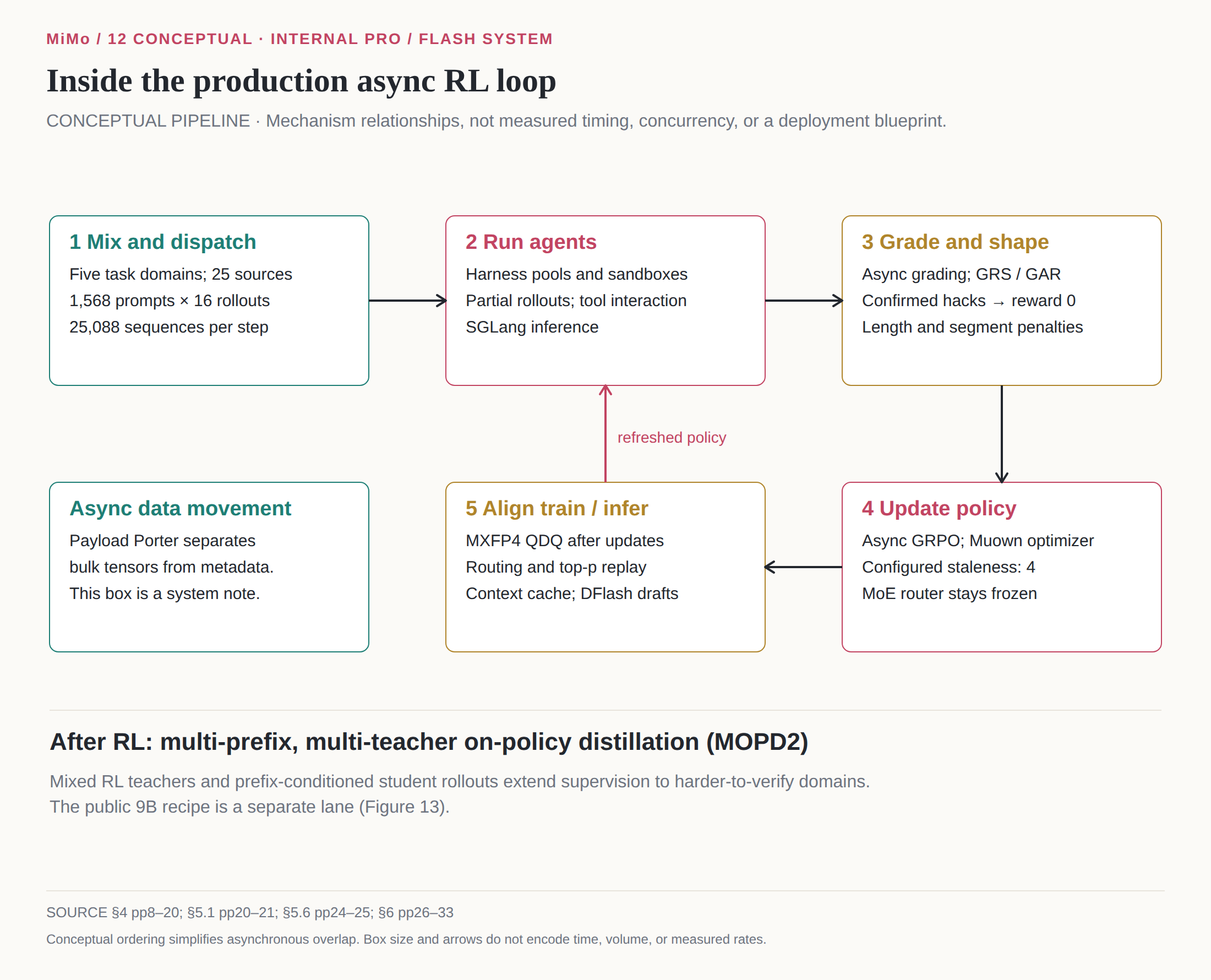
The diagram’s clean arrows conceal concurrency. Some agents are still working while other groups are graded. Some completed work may be carried forward. The policy can change before every sequence finishes. The training system has to decide what is old enough to discard, what can be resumed, what is waiting only on a grader, and what should be dispatched next to preserve the mixture.
This is why “one run” is a systems claim as much as an algorithmic one. A single mixed run avoids a particular sequence of domain-specialization stages, but it concentrates the scheduling problem. If the quick tasks finish first and monopolize retained batches, the intended task mixture exists only in a configuration file. The Sample Mixer, dynamic filtering and partial-rollout machinery are how Xiaomi tries to turn that configuration into the distribution the optimizer actually sees.
The equation only works if the history is true
The report writes its GRPO policy-gradient objective in a form that makes the bookkeeping visible. Using its notation, the essential expression is:
ℒ(θ) = −𝔼q ∼ ∪dDd, {oi} ∼ μ [ (1 / ∑j=1G|oj|) ∑i=1G ∑t=1|oi| ri,tMi,tAi log πθ(oi,t | q,oi,<t) ] (1)
Here q is the prompt; D_d is a domain’s task dataset; G is the group size, sixteen in the reported production run; and o_i is one sampled output sequence. The index t picks a token position. The trainable policy is π_θ, while μ denotes the rollout policy that supplied the data. M is a mask identifying positions eligible for the loss. A_i is the group-relative advantage assigned to the attempt, and r is an importance weight relating the current policy to the policy that generated the token. Report Eq. 1, pp8–9, and §5.1.
Read it as a request to make better-than-group attempts more likely and worse-than-group attempts less likely, using only eligible generated positions and correcting for policy mismatch. The leading minus sign turns that preference into a loss to minimize. The denominator is the sum of output lengths within the prompt group, not a separate inverse length for each rollout followed by division by G. Tokens are normalized within each prompt group, then prompt groups are averaged. Longer attempts can still contribute more tokens within their group; a longer group does not automatically receive more total weight than another prompt. That distinction matters when reproducing the reduction.
For an intuitive unnormalized group baseline, advantage has the form A_i = R_i − mean(R), with reward R_i compared against the other attempts at the prompt. Some GRPO variants divide by group standard deviation. The public Code recipe explicitly disables that normalization. It is important not to insert the textbook default into a source-specific explanation merely because the acronym is familiar.
The ratio can be written r = stop_gradient(π_θ/μ), evaluated on the generated token and its actual history. Stop-gradient means the weight is treated as fixed when differentiating that surrogate expression, rather than differentiating through the weight a second time. The report further describes clipping controls around this update. The expression above is not a claim that an unrestricted importance ratio is allowed to dictate arbitrarily large policy changes.
There are several places where “actual history” can go wrong. A tool reply may be accidentally included as a generated token. A reconstructed conversation may tokenize differently from the one used during rollout. A partial rollout may contain tokens from more than one policy version. A tool schema may change. The numerical distribution used for sampling may differ from the one used when recomputing probabilities. Each error damages the meaning of r or M. The math is compact because it assumes the system did not lose the evidence.
Production inference probabilities are kept from generation time rather than recomputed as if a partial rollout had been generated entirely by the latest policy. This is necessary because a long sequence may be interrupted for an update and resumed later. The old prefix is still part of the agent’s experience. Pretending its tokens came from the new policy would erase the off-policy distinction without making the data on-policy. Report p21.
The production clipping scheme has four independently controlled bounds: lower and upper bounds for positive-advantage tokens, and lower and upper bounds for negative-advantage tokens. Both sign-specific intervals begin at [0.2, 5.0]. Xiaomi describes adjusting them with policy entropy: widening positive and narrowing negative intervals when entropy is too low, with the opposite adjustment when it is too high. Direction-specific clipping rates are monitored. The report defines a mask that excludes ratios outside the interval for their advantage sign. These are ratio intervals, not a conventional shorthand for “plus or minus 0.2,” and not simply the public PPO-style clipped surrogate.
The inspected public vanilla loss is different. It clips using 1 − clip_ratio_low and 1 + clip_ratio_high, then applies a negative-advantage dual clip using clip_ratio_c. Code supplies 0.2, 0.2 and 3.0. A launch script with those values does not reproduce the report’s entropy-adjusted four-bound policy. Public loss implementation; Code inner recipe.
Production optimization uses a learning rate of 3 × 10⁻⁶, no warmup or weight decay, and gradient clipping at 1.0. The Muon portion uses momentum 0.95 with Nesterov enabled, ten Newton–Schulz iterations per update and an additional update scale of 0.5. Adam-managed parameters use β₁ = β₂ = 0.95 and ε = 10⁻⁸. The router is frozen. FP32 master weights and Muown row state are carried from the SFT checkpoint for MXFP4 stability. These are report values; the public Code actor instead defaults to learning rate 10⁻⁶ and weight decay 0.01. Report pp20–21; Code recipe.
That is a lot of detail for one update, but it prevents a misleading recipe: “GRPO, sixteen samples, go.” The algorithm name leaves out reduction semantics, clipping, numerical policy, parameter classes and age control. Those omissions are exactly where two nominal reproductions can cease to be the same experiment.
The slowest agent does not get to set the clock
Synchronous collection waits for a whole batch before updating. In long agent tasks, that gives the slowest sequences unusual power. A repository setup, a stubborn browser interaction or a late verifier can leave expensive training resources waiting for a handful of unfinished episodes.
The production approach uses asynchronous partial rollouts with a reported staleness setting of four. In-flight sequences can be interrupted at collection and resumed in a later rollout phase. The price is re-prefilling their context after a policy update, plus the statistical problem of learning from older behavior. Xiaomi argues that large batches help amortize the re-prefill cost. This is a trade, not a way of making waiting free. Report §§4.1, 5.1.
Staleness is a budget on how far rollout behavior can lag the training policy. It should not be confused with elapsed wall time. A trajectory that spends a long time in a tool could span few updates; a shorter one could cross more updates during a faster phase. Nor should a per-step average be mistaken for the worst individual trajectory.
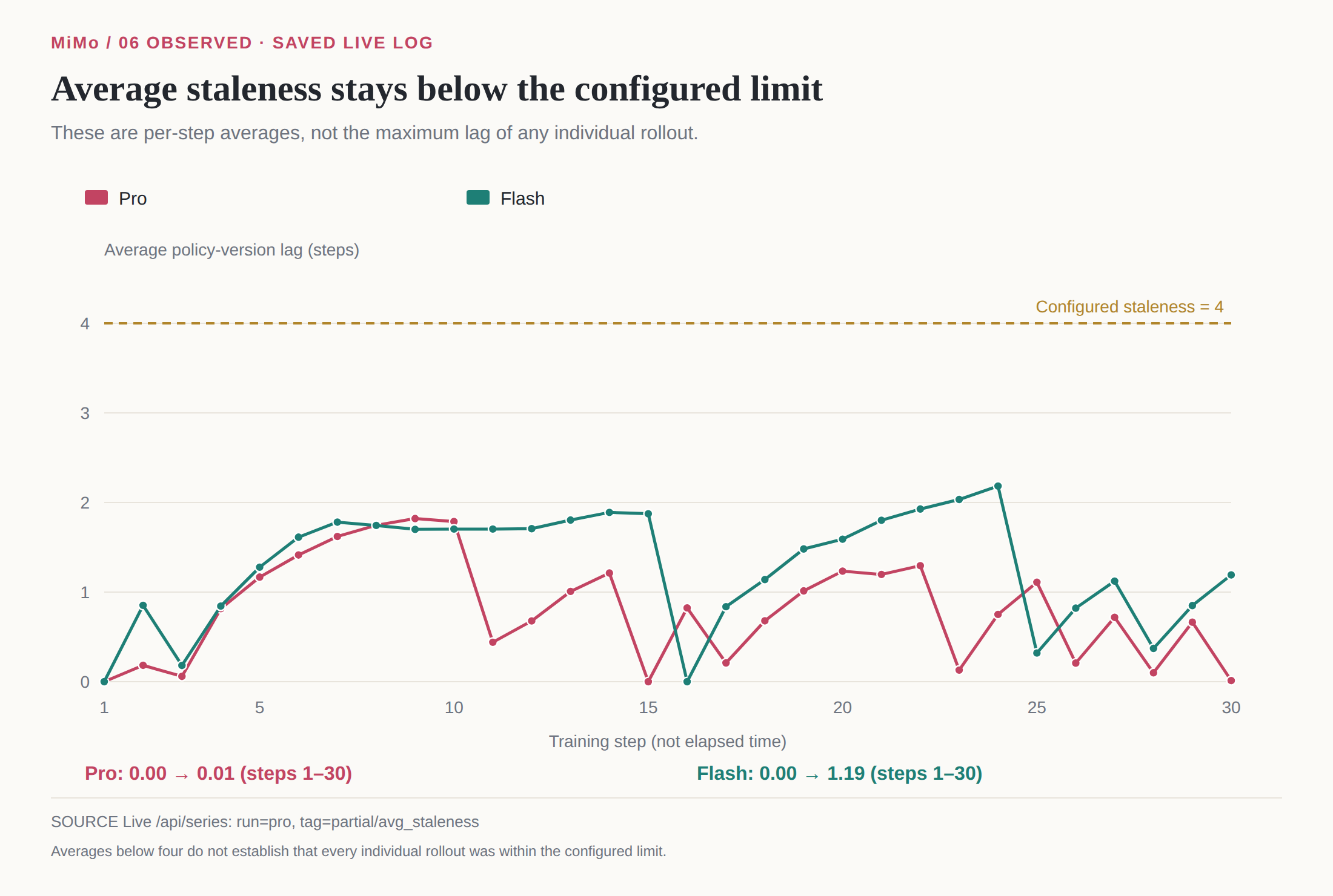
The largest saved averages are about 1.82 for Pro and 2.18 for Flash. They are below four. That supports a statement about the averages, not proof that every single sequence respected the bound. Individual age distributions would be needed for that stronger conclusion.
The public replay code uses its own explicit age definition. Its asynchronous stale-eviction predicate is global_steps − prompt_dispatch_step + 1 > threshold. This measures prompt-dispatch age, not precisely the same thing as per-generation policy-version lag. Code’s outer launcher defaults to threshold two and drop; Cyber uses eight and drop; Visual and Music YAML use four and drop. General has asynchronous generation but a synchronous trainer mode. “Async” is not one switch shared uniformly by the release. Replay age checks; public launchers.
Dynamic group filtering adds another complication. A group with no usable reward contrast contributes little to a group-relative update. The inspected DAPO-style classifier considers non-infrastructure rows, and treats no valid rows, one valid row or zero standard deviation as lacking usable contrast. That includes more than binary all-pass or all-fail groups. A continuous-reward group whose members all receive the same value can be equally uninformative.
Filtering improves the density of comparative signal, but changes the relationship between dispatched and retained data. If one source produces many no-contrast groups, it needs more rollout attempts to meet its retained quota. If infrastructure errors are incorrectly counted as model failures, both filtering and scheduler estimates become distorted. The scheduler is not merely keeping GPUs busy. It is helping decide which training distribution exists.
A passing test is the beginning of grading
A test suite can tell you that a patch passed the tests it ran. It cannot automatically tell you that the patch was precise, maintainable, free of unintended behavior, or produced without reading a leaked solution. RL tends to discover this distinction faster than launch copy admits.
MiMo’s report divides its coding grading work into Groupwise Reward Synthesis, GRS, and Groupwise Advantage Redistribution, GAR. They are related but not interchangeable. GRS produces reusable rubrics offline for a selected high-pass-rate subset. GAR inspects a rollout group online and redistributes learning signal among passing attempts. Both add judgment beyond a binary test result. Report §4.3.
For GRS, an agent studies multiple offline rollouts together with the task specification and repository, then builds solution and behavior rubrics. During training, a grader enters the execution environment and scores against those rubrics. Reward is multiplicative:
Ri = Ritest Sisol Sibeh (2)
R_test is the binary test result. S_sol is a solution-quality score, and S_beh is a behavior score. A failed test remains zero regardless of how appealing the grader finds the rest. Among passing attempts, quality can reduce reward. The product encodes a hierarchy: correctness is a gate, not just another weighted preference that a stylish failure can compensate for.
GAR instead uses an SFT-trained agentic grader to inspect a mixed-outcome group in a shared workspace. It can inspect the repository and run tests. Passing patches are assessed along five dimensions: approach suitability, precision, minimality, absence of unintended effects and craftsmanship. The grader can identify a patch that technically passes by weakening validation, swallowing exceptions or adding speculative compatibility branches. Those are exactly the changes that can look productive in a narrow score and become a maintenance headache later.
Let P be the passing set after confirmed hacks have been corrected to zero reward. Let f_i, between zero and one, represent the quality factor assigned to passing attempt i. The report’s redistribution is:
λ = (∑j∈PAj) / (∑j∈PfjAj)
A′i = λfiAi if i ∈ P; otherwise Ai. (3)
The plain reading is “move more of the positive teaching signal toward the better passing solutions without casually changing the total budget allocated to passes.” In the uncapped form, summing the revised advantages over P recovers the original sum by construction. In practice λ is capped, the group mean is re-subtracted, and the resulting scalar advantages are broadcast to response tokens. The exact numerical mapping from grader ranking to f_i is not fully specified in the report. We should not manufacture it.
The grader runs asynchronously. Unusable grading outputs fall back to original advantages in the reported design. That makes sense as an availability trade: losing a quality judgment need not erase an otherwise valid executable result. But it also means grader reliability affects the effective objective. A run whose advanced grading frequently fails is not receiving the same signal as one whose grader succeeds consistently, even if the policy optimizer config is identical.
Xiaomi’s GAR ablation supports the mechanism without proving every broader claim one might want. It is a code-only Flash experiment with batch 128, token-mean loss and a run through step 52, not the main mixed-domain prompt-mean production experiment. Without GAR, turns and tokens grow quickly, length-limit hits increase and pass-rate improvements stall. With GAR, turns remain steadier and gains continue. Maintainer audits describe more precise patches in the GAR condition. Report Figure 8, pp18–19.
The saved evidence does not provide trustworthy interior numeric points for those curves. There is no recreated GAR learning curve in this article. Drawing a smooth invented line would make the presentation prettier by weakening the evidence. The report’s qualitative account and the stated experimental setup are enough to explain what was tested.
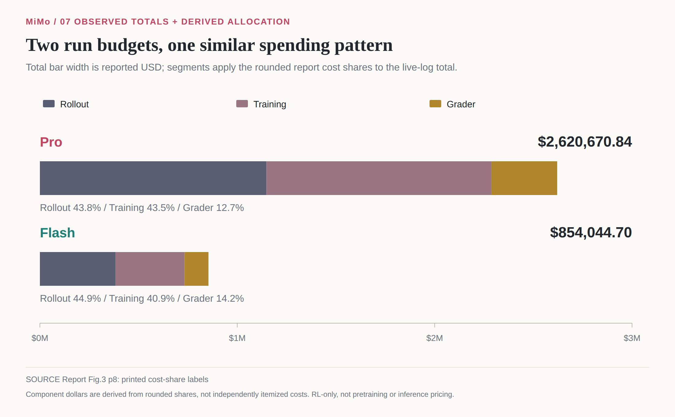
The grader share is the visible price of treating evaluation as work. It is not enough to budget only actor updates and generated tokens. A system that opens environments, checks behavior and compares solutions consumes its own compute and service capacity. A faster learner with an unreliable grader can learn the wrong lesson faster. The accounting recognizes that uncomfortable possibility.
Shorter is not always better, and punishment has a budget
Long trajectories can represent useful persistence. They can also represent repetition, failed tool calls and a model trying every imaginable workaround until a verifier finally says yes. A blunt length penalty risks suppressing the first behavior along with the second.
The report therefore defines a group-relative length penalty that operates only when a group’s pass rate exceeds a gate A. It selects a reference length ℓ*_q from the B-th percentile of successful rollouts for prompt q. Successful attempts that exceed that reference by more than a tolerated relative margin δ incur a deduction, capped at X. Failed attempts are not the target of this particular efficiency penalty. Report Eq. 4.
A numerically clear equivalent form, making the nonnegative ramp explicit, is:
zi = clip((ℓi/ℓq★ − 1 − δ)/(s − δ), 0, 1)
R̃i = Ri − 𝟙[i ∈ Pq] Xziγ, when |Pq|/G > A. (4)
ℓ_i is generated length; P_q is the passing subset; s is the relative excess at which the penalty saturates; γ controls the shape of the ramp. This writes the clipping before a possibly noninteger exponent so negative excess cannot become an invalid fractional power. Below the tolerated excess, the deduction is zero. Above saturation, it is X. Between them, the curve controls how gently or sharply waste becomes costly.
The rationale is comparative rather than ascetic. If nobody can solve the task, punishing long attempts may choke off exploration. If enough attempts succeed, successful peers provide evidence about how much work the task plausibly needs. That evidence is still imperfect: a shorter passing rollout might have been lucky or used a fragile shortcut. Length shaping complements quality grading; it does not replace it.
Segment-level behavioral penalties act later, on advantages rather than only on scalar rewards. Let h_i,t mark a flagged token or segment, κ > 1 strengthen negative signal on flagged positions, α scale clean positive positions, and β scale clean negative positions. The placement of the negative-branch scales matters:
Ãi,t =
α(1 − hi,t)Ai, if Ai > 0
[β(1 − hi,t) + κhi,t]Ai, if Ai < 0
0, if Ai = 0. (5)
Positive flagged tokens lose their positive advantage. Clean positive tokens are scaled upward to compensate where possible. Negative flagged tokens are multiplied by κ; only clean negative tokens are scaled by β. Putting β outside the entire negative expression would also scale the flagged negatives, which is not the described or inspected operation. Report p20; signed rebalance implementation.
For flagged and clean token sets H and C, separated by advantage sign, the ideal compensating scales are:
α = min(αmax, 1 + ∑H+A / ∑C+A)
β = max(βmin, 1 − (κ − 1) ∑H−|A| / ∑C−|A|)
This tries to preserve positive and negative advantage mass separately. It does not promise that the final gradient vector is unchanged: different token gradients point in different directions, and the whole purpose is to change which behavior receives credit. “Mass” here is the sum of advantage weights, with appropriate token weighting where used, not a conservation law for the optimizer’s parameter update.
Nor is mass conservation unconditional. If there are no clean tokens to receive redistributed weight, a denominator vanishes. If α hits its cap or β its floor, compensation is incomplete. The public implementation logs imbalance and skips the conservation assertion on clamped sides. The honest claim is a conservation-oriented design with explicit failure conditions, not an invariant that survives every possible group.
The public Cyber reference makes this tangible. It supplies κ = 2, α_max = 2 and β_min = 0.5. Its length settings include maximum deduction 0.2, exponent 1.5, deadzone zero, saturation one, a 0.3 quantile anchor and a pass-rate gate of 0.5. Length metrics include turns, input tokens and output tokens, combined by their maximum. These are public reference-recipe constants, not recovered secrets of the production run. The report leaves its production values unpublished. ARVO reference profile.
One final distinction prevents a quiet error. General’s YAML also configures length shaping, but the source review did not identify a consumer for that algorithm key in the inspected trainer path. The visible shaping call is gated through the ARVO reference-penalty mechanism. General’s settings are therefore configured-only, with application unconfirmed. A parameter can be beautifully documented and still not reach the loss. That is precisely why source tracing is part of this story.
The environment can accidentally hand out the answer
A repository is not an inert prompt. It is a filesystem with history, caches, installed packages, network access and executable tools. Any one of those can turn “solve this issue” into “find where the solution was left.” In agentic RL, environment preparation is part of reward design.
The report describes five coding-task synthesis pathways, alongside pipelines for general tool tasks, visual work and cybersecurity environments. The common requirement is more demanding than producing plausible instructions: the task needs a starting state, a useful objective, an executable environment and a way to judge success that does not expose the answer during the attempt. Task synthesis and verifier synthesis have to agree about what completion means. Report §4.2.
The five coding pathways cover different sources of difficulty. GitHub-based construction collects pull requests and associated issues, filtering duplicates, malformed candidates and irreproducible tasks. A sufficiently complete issue can supply the specification directly; otherwise a model reconstructs an issue-style request from the reference patch and repository context, with instructions to avoid implementation details that reveal the solution. The second route uses real development requests, including feature work, refactoring, debugging and maintenance, with generated tests intended to operationalize the requested behavior.
Specification-driven tasks emphasize detailed, multi-constraint requirements. Source-code-driven synthesis uses CodeMidas to recover observable functionality from existing repositories, so a task need not depend on a conveniently written issue or pull request. Long-horizon construction iteratively expands requirements and introduces dependencies across components, with tests for the resulting multi-step behavior. Public sources and licensed data supplement the distribution. These are reported construction methods, not five labels inferred from the public parquet counts. Report §4.2.1, pp9–11.
The supervision checks are as important as the synthesis. Tests should accept implementations satisfying the stated requirement without requiring incidental details of the reference patch. Xiaomi describes four attempts per task, then an auditing agent with access to the specification, tests, reference patch and all four submitted patches, outputs and conversation logs. A passing solution judged incorrect suggests a false positive in verification; a failing solution judged correct suggests an overrestrictive test or an execution problem. The disagreement directs review rather than being resolved automatically in favor of either the test or the judge.
For tasks with a reference patch, fail-to-pass tests should fail before the patch while pass-to-pass tests already pass. After the patch, both sets should pass. The report requires these outcomes to remain stable across eight reruns, screening out flakiness and environmental variability. This does not prove that the verifier captures every possible correct solution, but it checks more than whether the reference patch happened to work once. A noisy verifier turns identical behavior into inconsistent teaching; an overrestrictive verifier can punish a valid alternative implementation.
General environment synthesis pursues a related compromise. Real files and local software mocks reproduce supported operations, state changes, output formats and errors; tools that already work locally can be integrated directly. Keeping state local and resetting each rollout to a fixed starting point reduces dependence on changing external services. The cost is a fidelity question: a model can learn a mock’s behavior without that mock perfectly representing the real application. Resetability improves the experiment’s control, not automatically its transfer to every live workflow. Report §4.2.2.
For general tasks, the environment can include structured enterprise-like state, tools and a collection of atomic rubric checks. Some checks are executable; others require a model judgment. A task that asks for a state change should be graded against the state, not merely against an agent’s final claim that it made the change. If a model judge is used, its inputs and rubric become another interface that needs versioning and scrutiny. The report uses a self-hosted MiMo-V2.6-SFT grader for general tasks during production RL, which should not be confused with the separate default model name in the public General launcher.
Visual tasks include open-ended design and high-fidelity replication. These have different evidence requirements. Replication can compare an output with a target. Open-ended design has no single pixel-perfect answer, so relative aesthetic quality and requirement satisfaction need their own judgments. A screenshot can show beauty while hiding a broken interaction. A runtime check can show that a page loads while saying little about whether its layout answers the request. The public visual grader later makes that separation explicit.
Cybersecurity tasks are built around known fuzzing failures and controlled environments. The reported oracle matches vulnerability type and the topmost project-level stack frame from a sanitizer report. The description and verification target come from the same report, reducing disagreement between a natural-language description and the failure being checked. This is a deterministic task oracle, not a guarantee that every security property of a program has been assessed. Xiaomi also notes corrected CyberGym environments in its evaluation procedure, a caveat that matters when comparing numbers across papers. Report §4.2.4 and §5.2.
The saved release inventory records 7,780 rows across five parquets: 2,698 Code, 2,093 Webdev, 1,000 Cyber, 1,000 Music and 989 General. It also records 925 materialized General environment directories. Those are different units. A parquet row count is not a count of fully inspected containers, and a directory count is not proof that every referenced task bundle is ready to launch. The public dataset gives the inventory a concrete home without removing the need to check each dependency.
Likewise, the saved registry inventory reports 3,764 Docker tags. A capped page of 1,000 tags contained 699 arvo-v1 tags, 236 format-code-task tags and 65 general-agent-env tags. That page is not the whole registry, and tags are not necessarily unique image contents. No image interiors were downloaded or audited for this article. A release can be materially larger than a README while still being only partially inspected.
The report’s reward-hacking examples are painfully ordinary software actions used in the wrong context: installing a package and reading a later test suite, fetching a fixed upstream source file, cloning an upstream repository, consulting an issue tracker ticket, checking available package versions. The problem is not that package management or repository browsing is inherently bad. The problem is that a benchmark’s intended information boundary can make those actions shortcuts to privileged answers.
Xiaomi describes a layered defense. Mid-training includes reflection corrections. Environment preparation removes artifacts and history and constrains network access. A dedicated Hack Agent adversarially screens tasks. Offline training-trajectory audits look for new patterns. A groupwise grader resets confirmed hacks to zero reward before group statistics are recomputed. The reported confirmed-hack share stays below two percent of trajectories for both production models. That is a measured share of confirmed cases under the described detection process, not a proof that undetected reward hacking is below two percent. Report §4.2.6.
The public source contains concrete measures in the same direction. Hidden tests are supplied through a test patch applied at reward time rather than sitting in the rollout workspace. Git history stripping accounts for cruft packs. Answer-leak domains can be blocked through host mappings. The anti-hack guard uses patterns derived from 6,026 judged hacking trajectories. The DeepSWE path grades in a fresh second pod rather than trusting the agent’s worktree, caches and tests after an unrestricted editing session. These findings come from the earlier implementation review, not a new end-to-end execution here. Public verifier source; mimoagent source.
A source comment gets the threat model exactly right: “anything present during the rollout is readable with cat.” Hiding a test by convention inside a writable environment is not hiding it from an agent with shell access. Another comment refuses to treat a partially applied test suite as a valid verdict. That refusal is good engineering: an explicit testbed failure is preferable to a confidently wrong reward.
The anti-hack interceptor can block a suspicious action before dispatch and return a bland denial rather than destabilizing the trajectory with an entirely new failure protocol. This is not proof of complete security. Pattern matching has blind spots; host-file blocking is not a full network policy; a fresh grading pod still needs a trustworthy image and correctly transferred patch. The point is that the code treats contamination as a live design problem instead of assuming the model will politely stay inside the experiment’s intention.
They took away the router’s second steering wheel
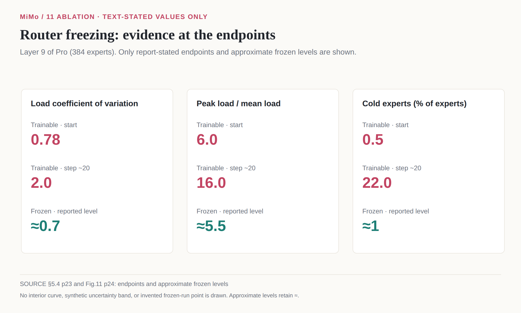
The router ablation is the cleanest detective story in the report. During RL with a trainable router, expert loads drifted. In the reported layer-nine analysis, the coefficient of variation rose from 0.78 to 2.0. Peak expert load rose from six times the mean to sixteen times. The share of cold experts rose from 0.5 percent to 22 percent over the early training span. Report §5.4.
Coefficient of variation is standard deviation divided by mean; it measures relative dispersion. Peak-to-mean load describes the most overloaded expert. “Cold” here means below a tenth of mean load. These are complementary diagnostics. A single hot expert can create a memory or latency problem; many cold experts indicate that capacity is being left unused. A benchmark score alone would not tell you which of these is happening.
The team then restored the step-twenty router parameters to their pre-RL values. Load balance recovered while benchmark performance remained unchanged in the reported experiment. That intervention is stronger evidence than a correlation between training time and imbalance. It points to router drift rather than degraded expert weights as the cause of the load problem.
The fix was to freeze the router during RL. The frozen condition kept the coefficient of variation near 0.7, peak load around 5.5 times the mean and cold experts around one percent, while benchmark improvements continued. The implication is not that router learning is always bad. It is that this stage’s reward-driven updates could distort routing without supplying the capability benefit needed to justify the systems cost.
There is a subtle limit to the fix. Freezing parameters does not freeze which tokens appear in a batch. Different inputs can still route unevenly through a fixed router. In the Pro production run, an expert-parallel rank reportedly exceeded thirty times the mean token load at one layer, producing an out-of-memory failure around step seventeen. The recovery adjusted parallelism; it did not undo the router-freeze decision. Report §5.5; run notices.
That is a useful distinction between distributional drift and batch-local imbalance. The ablation addresses a learned routing policy becoming progressively concentrated. The OOM shows that even stable routing can meet an unfortunate token distribution and an insufficient capacity arrangement. A global load chart and a micro-batch memory budget answer different questions.
Public code supports the existence of both freezing and routing replay. The model initializer sets selected MoE router weights to requires_grad=False. The Megatron engine consumes routed-expert metadata, checks R3 replay mode, builds a response replay mask and installs replay data. These are inspected framework capabilities. They do not establish that all production routing machinery is released or that the dense public student exercises it. MoE initializer; Megatron replay path.
I would rather have that precise answer than either slogan. “The production code is all missing” is false. “The production system is fully reproduced by the public recipe” is unsupported. The release is more useful when we resist both.
A trajectory is not one long chat string
The production report gives its agent data four levels: Sample, Sequence, Context and Segment. A Sample is the dispatched prompt group, accepted or rejected as a group for GRPO. A Sequence is one execution of an agent loop. A Context is a dialogue branch within that execution. A Segment is a turn. Report §6.1.
This hierarchy handles behavior that a flat transcript cannot describe cleanly. An agent may spawn a subtask, maintain separate roles or compact a history. Those can produce multiple contexts inside one sequence. Prefix matching and cache reuse happen at the context level. Behavioral violations may occur only in particular segments. Group selection happens at the sample level. If those units are collapsed into “the response,” masking and credit assignment become ambiguous.
Only model-generated turns belong in the policy loss. Tool observations and other supplied content still consume context and influence subsequent generation, but they are not actions sampled by the policy. Training on them as if they were generated decisions would teach the model to imitate its environment rather than improve its behavior within that environment.
The reported Penalty Module separates a rule from a strategy. A rule detects something: unavailable tools, garbled tokens, repetition, infrastructure failure or another condition. A strategy decides what to do: monitor it, mask data, shape advantage or stop an execution. The hierarchy gives an escalation path. A context without surviving turns can be dropped; a sequence can lose usable advantage; a sample can be rejected. This is more expressive than assigning every suspicious episode a scalar minus one.
It is also easier to get wrong. A benign formatting problem, an actual tool mistake and a failed network should not all teach the same lesson. If a pod never started, the model did not choose the bad action that caused the failure. If a generated tool call was malformed, it did. The distinction must survive serialization into the fields the trainer actually reads, not merely appear in an exception message for a log viewer.
The production execution pool uses persistent multi-tenant Ray actors rather than creating a heavyweight control-plane object for every agent loop. Many loops share an event loop; blocking operations go to background threads. Separate codebases can occupy separate pools, with a fixed host-actor budget at startup. The report describes this partly as a response to control-plane pressure, including file-descriptor exhaustion. The training system is managing millions of pieces of work without wanting millions of expensive orchestration objects. Report §6.2.
Payload Porter separates control information from bulk data. The driver deals in rewards, lengths and payload keys; the full payload is written once to a distributed store such as Ray’s object store or TransferQueue. Packing workers fetch the rows they need for their tensor- and context-parallel responsibilities. Multimodal metadata and pixels can travel separately, with incremental transport for newly added observations.
This is not glamorous, which is why it deserves space. A browser trajectory can accumulate gigabytes of screenshots. Passing the whole growing payload through a central Python driver on every turn would make the driver a data ferry rather than a coordinator. Separating data and control paths reduces that pressure, though the report still records a later CPU packing OOM. Better architecture reduces bottlenecks; it does not abolish finite memory.
The mixer has to buy the batch it promised
Across the report’s 25 profiled data sources, average generated-token counts vary by ninety times and active rollout duration by sixty-six times. A uniform launch count cannot deliver a uniform retained mixture under that heterogeneity. Long tasks need more concurrent work in flight; low-acceptance tasks need more attempts. Report §6.3.
For source i, let B_i be its target retained groups per step, r_i its estimated acceptance rate and t_i its active rollout duration. Expected generation demand is m_i = B_i/r_i. This is an estimate of how much work must be attempted to retain the desired amount. If acceptance deteriorates, m_i rises even when the desired training share has not changed.
The report’s oversampling rule is:
pi = clip(cti − 1, pmin, pmax), with (∑imipi) / (∑imi) = p̄. (6)
p_i is a source-specific oversampling ratio. The shared coefficient c is chosen to meet the weighted average oversampling budget p̄, subject to lower and upper bounds. Longer sources receive more headroom, but not without a global budget or per-source caps. The report does not publish all those bounds, so the equation is a policy description rather than a fully reconstructible configuration.
Scheduling then blends steady target demand with the current deficit:
wi = α Bi/ri + (1 − α) [(Bi − Ai)/ri]+. (7)
A_i in this equation is the already accepted count for source i, not the policy advantage used earlier. The positive-part operation clips negative deficit to zero. The first term keeps attention on long-run demand; the second prioritizes sources still short of their current quota. At steady state the report uses α = 0.5. This α is a scheduling mixture weight, not the positive-token redistribution scale from Eq. 5.
Those overloaded letters are worth spelling out because the concepts differ. Policy advantage answers “was this attempt better than its peers?” Accepted count answers “have we collected enough from this source?” A system needs both, but confusing them would turn a mathematical explanation into decorative notation.
Predictive dispatch tries to start work before the collection step needs it. Sample replay helps the first collection after startup or recovery, reusing eligible completed work within source-specific staleness limits. The report describes a startup collection slowdown of about 1.8 times relative to continuous operation. That is a reminder that a warm pipeline and a newly restarted one are not the same queueing system.
Startup estimates can be biased because short rollouts finish first. If the scheduler treats those early completions as representative, it may dispatch too aggressively or allocate the wrong balance of resources. The report connects such startup bias to exhaustion of both GPU and pinned-host cache pools. Another failure involved one interaction loop producing much shorter rollouts than others on the same coding dataset, skewing early steps after restart. The scheduler was seeing a changing distribution, not simply a slow machine.
The lesson is practical: a target mixture is an obligation the runtime has to keep paying for. You cannot verify it solely by reading dataset weights. You need accepted counts, filtered counts, carryover, durations, age and failure categories. Otherwise the training run can quietly become a curriculum chosen by whichever environments happen to finish first.
Training and inference must agree about the action
An importance ratio compares probabilities. It cannot correct a mismatch it was never told about. If rollout uses one numerical implementation, routing path or sampling support while training evaluates another, the ratio may partly measure implementation differences rather than policy change.
The report describes several consistency mechanisms aimed at that problem. Quantize–dequantize alignment after each update respects the MXFP4 Humming GEMM numerical constraints. R3 replays expert-routing choices from rollout. Top-p candidate replay preserves the truncated candidate support used when sampling. Together these address different reasons the training computation might disagree with the action-generation computation. Report §6.4.
Top-p truncation is especially easy to forget. Sampling is not always performed from the model’s entire raw vocabulary distribution. A nucleus can restrict the candidate set and renormalize probability over that set. If training later compares an untruncated probability with a rollout probability normalized over a small candidate set, the two quantities are not directly the same distribution. The report describes storing candidate information, initially as a vocabulary-width bitmap and later in sparse form. At top-p 0.97, the typical candidate set averages fewer than five tokens in the reported setting. That is a property of this run’s distributions, not a universal promise for top-p 0.97.
Routing replay has a parallel motivation. A sparse model’s chosen experts influence the computation that produced a token. Replaying that choice can reduce train/inference mismatch. Freezing router weights helps with drift, but it does not make replay conceptually redundant: numerical and execution differences can still affect routing behavior. The public framework’s R3 path is evidence that the release contains relevant support, while the report supplies the account of production use.
The Context Cache deals with another mismatch: the model’s need for a cache versus the agent’s habit of doing nothing on the GPU while waiting for a tool. During GPU execution, cache data lives in high-bandwidth device memory. During tool time it can move to a pinned-host pool, using side CUDA streams for transfer. Persistent per-context keys preserve the connection across turns. This creates a memory hierarchy suited to intermittent inference rather than permanently resident chat streams.
Pinned host memory is still memory. A scheduling error that admits too many long contexts can exhaust it just as surely as it can exhaust HBM. Moving a bottleneck off the GPU does not remove the need to measure it. The startup failures described in the report make that point more convincingly than a generic warning ever could.
DFlash drafting is tuned on RL rollout logs resampled toward the RL distribution. The report compares a block-six configuration with inherited MTP behavior and a block-eight alternative. It reports a 31.3 percent increase in average accepted length relative to MTP, about six percent higher global throughput for block six than block eight, and about 10.3 percent higher per-node throughput with FP8 drafting. Those are separate comparisons with different denominators. They should not be multiplied into one invented speedup. Report pp32–33.
CPU-resident optimizer states, fused loss kernels and bounded SWA context-parallel traffic round out the systems account. The fused kernels cover policy-gradient work, optional top-p renormalization, distillation loss and several metrics. Each optimization addresses a repeated cost in the loop. None alone explains the final capability gains. Their collective purpose is to make a large, awkward batch arrive often enough, and faithfully enough, for the optimizer to use it.
The dashboard is allowed to be messy
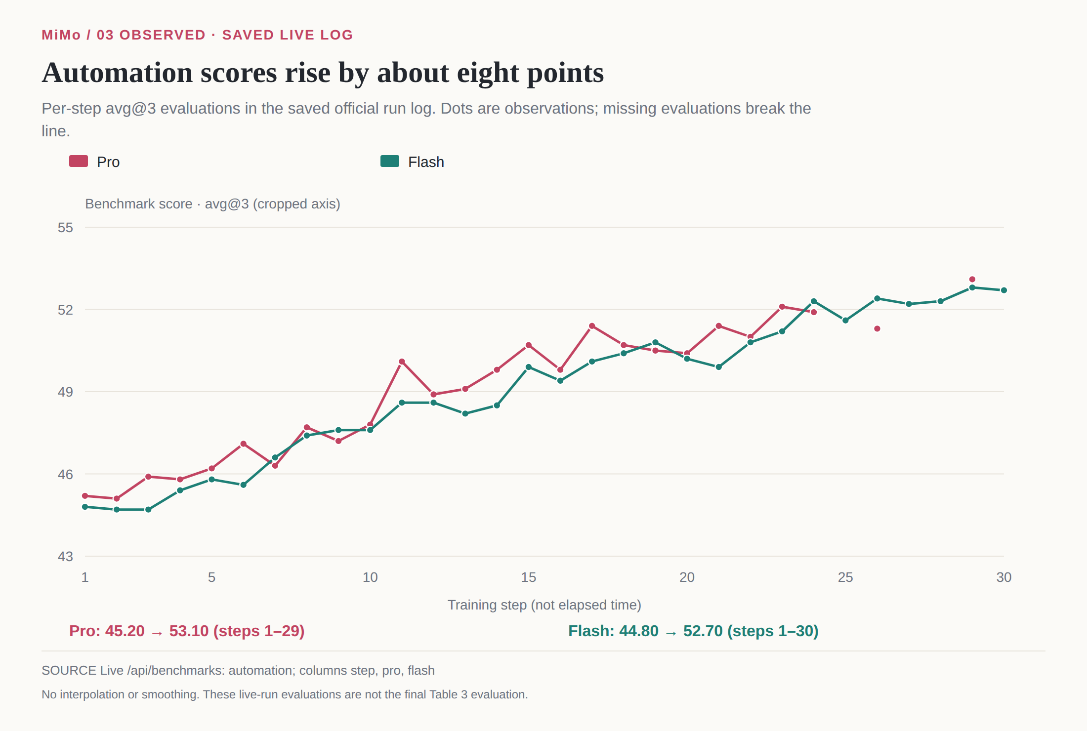
The saved live series are more useful when read as telemetry than as an animated victory lap. They show improvement, but also noise, missing evaluations, changing workload and interruptions. The charts here use saved observations rather than interpolated report curves.
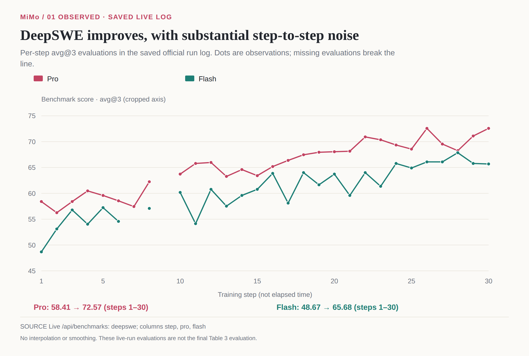
DeepSWE improves from the first posted evaluation to the last for both models. It does not improve at every step. Flash’s highest saved value is not its final one. Pro lacks a step-nine evaluation in this series; Flash lacks steps seven and nine. Leaving breaks in the line is a small but useful courtesy to the reader: the chart is not pretending to know what happened where no evaluation was saved.
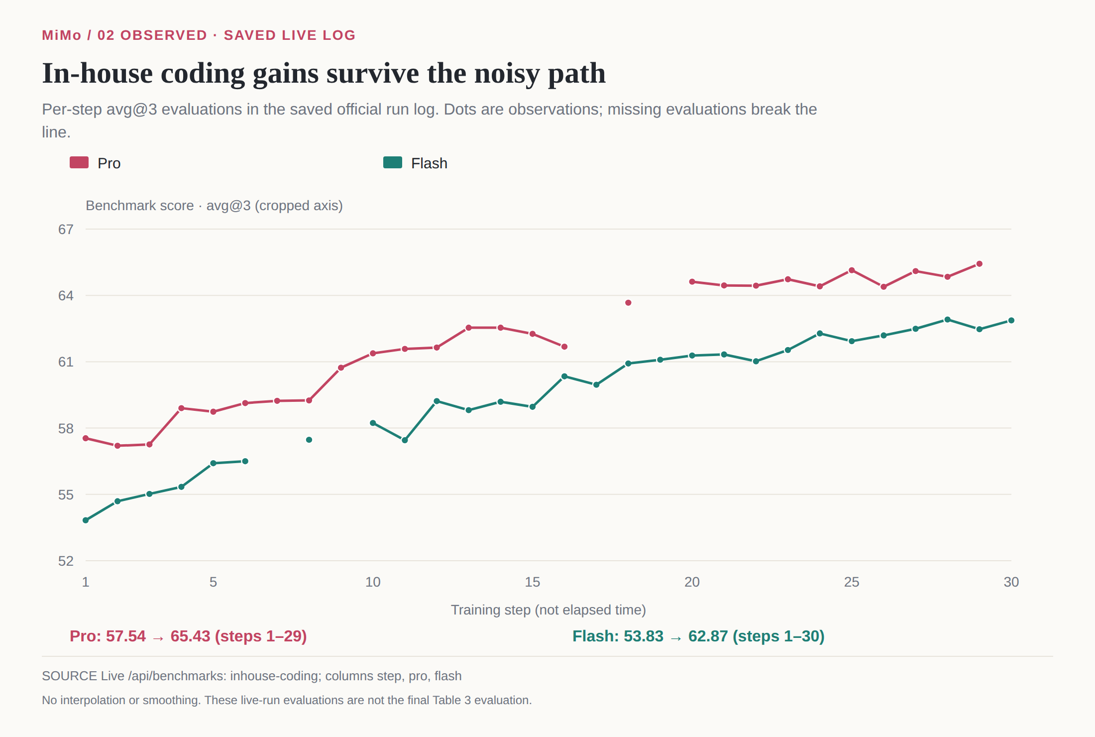
The in-house coding series offers a second view, but not an independently reproduced benchmark. Its value is the progression under the publisher’s evaluation process. The endpoint mismatch is harmless when labeled and misleading when silently forced into a common final step.
The training-task pass-rate series needs even more care. The metric dynsam/avg@n is a dynamic-sampler training statistic, not a fixed held-out benchmark. Task filtering and mixture changes can affect it. Its endpoint improvement is worth reporting, but it is not a clean causal estimate of generalization by itself.
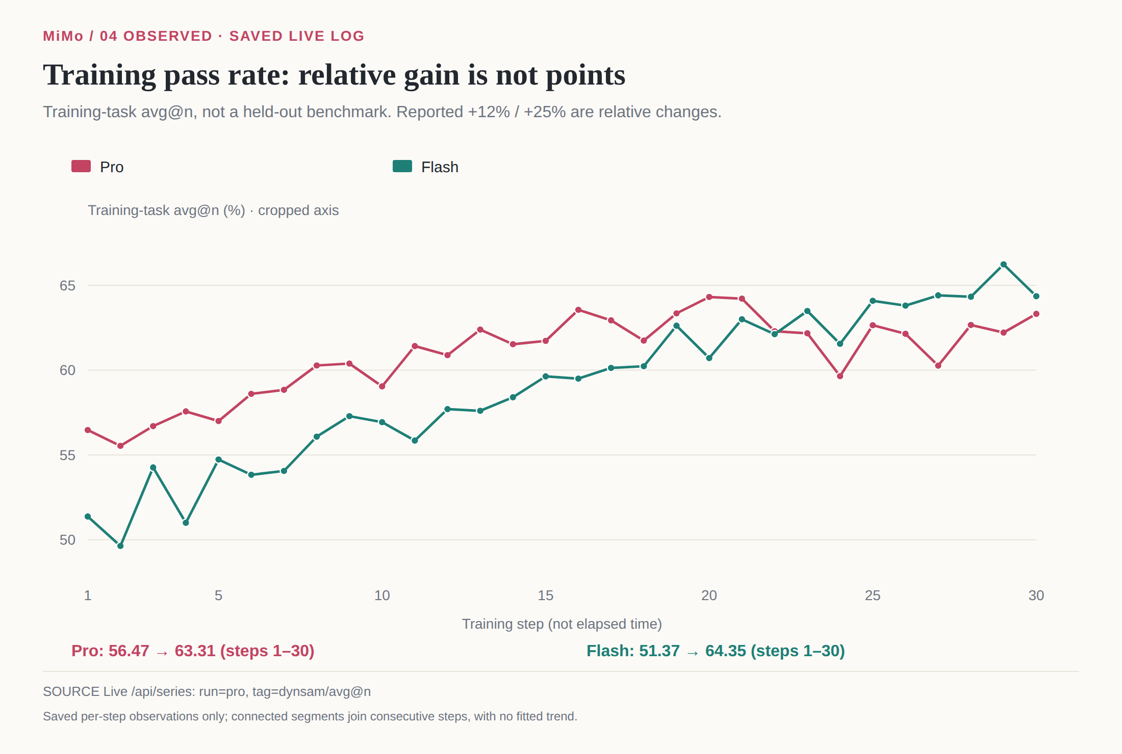
Using the saved unrounded endpoints, Pro’s relative change is (0.633138 / 0.564662 − 1) × 100, about 12.13 percent. Flash’s is (0.643526 / 0.513693 − 1) × 100, about 25.27 percent. Those are relative changes, not percentage-point gains. The subtraction of one is essential: a ratio alone describes the endpoint as a share of the starting value, not the increase. Both calculations use the saved observations before rounding.
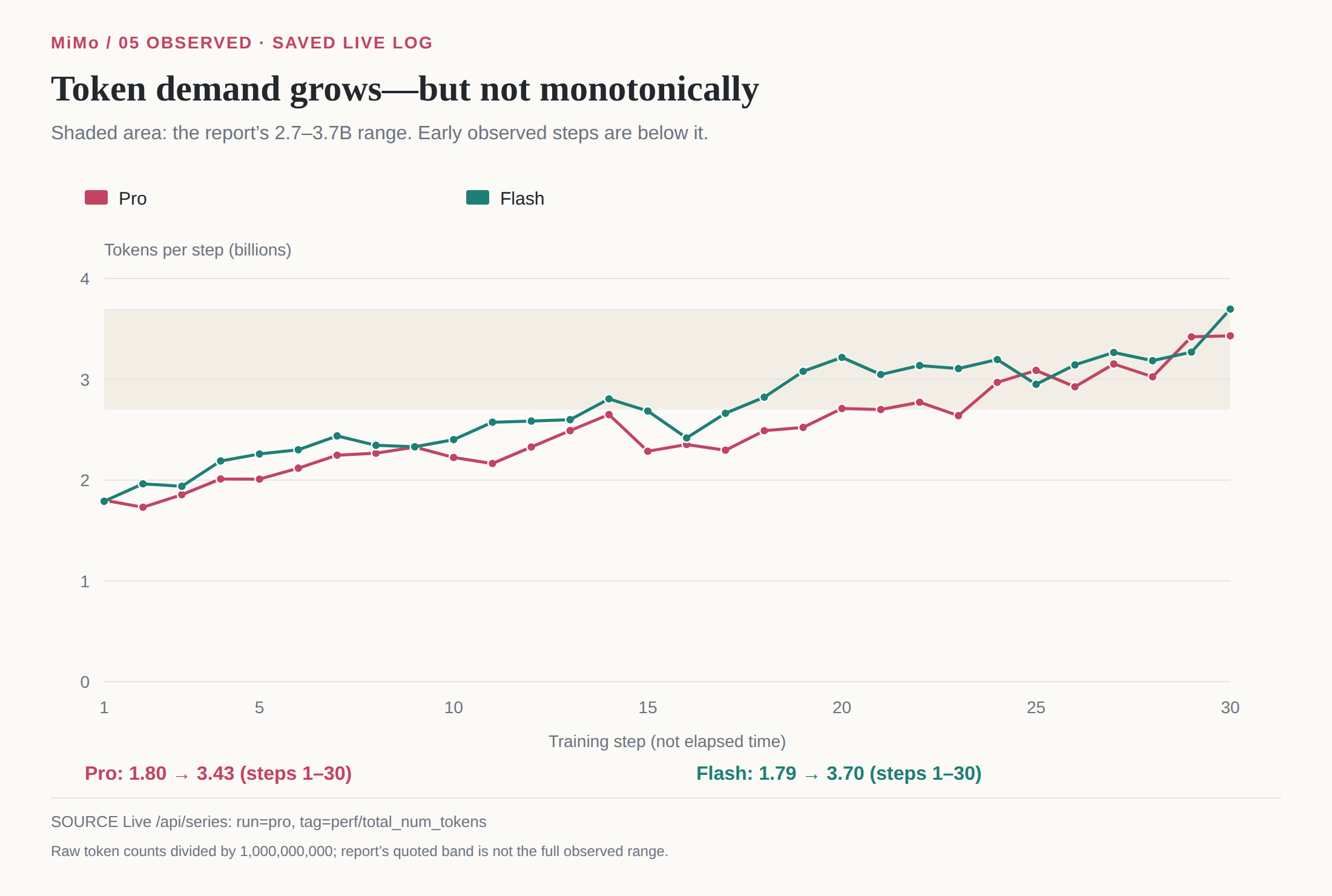
The token series exposes a real discrepancy in presentation. The report quotes 2.7–3.7 billion tokens per step; the saved live series includes smaller early steps and is nonmonotonic. We should say exactly that. It is not defensible to call the report range the full observed range, or to tell a smooth story in which tokens rise every step because the model steadily chooses harder problems.
Mean context endpoints also rise, from roughly 72.2K to 137.2K for Pro and 71.6K to 147.8K for Flash. That is consistent with a larger late-run token workload, but does not isolate a cause. Longer successful reasoning, more tool output, task-mix changes and inefficient behavior can all affect length. A causal explanation would require more than two endpoints and a pleasing narrative.
The entropy metric increases at the endpoints, from about 0.395 to 0.462 for Pro and 0.413 to 0.471 for Flash. This is an observation, not proof that the policy became more creative or that entropy control alone caused the gains. The step-timing series also changes substantially. Such telemetry can suggest questions for an experiment; it cannot answer every question merely because its field names look scientific.
Cumulative trained sequences reconcile cleanly: thirty steps × 25,088 sequences = 752,640 per run. That is not the number of distinct prompts, every sandbox ever started, or all generated work before filtering. The report’s wall-time totals should also stay separate from the live cost counter’s timing basis. Multiplying a displayed dollar-per-second rate by a rounded duration and demanding the exact invoice would impose an accounting definition the evidence does not establish.
The restarts are not an embarrassing footnote. The saved counters show fourteen for Pro and five for Flash. The report names GPU memory errors, Kubernetes failures, unreachable grading, routing-related OOM, cache pressure and CPU packing exhaustion. One notice describes hours of infrastructure errors on a dataset going undetected before a Flash restart. These disclosures make the run more interpretable: a bad reward can come from a bad policy, but it can also come from a broken testbed that nobody noticed quickly enough. Report §5.5; live notices.
The evidence still has holes. Several actor-loss, gradient-norm and train/inference-KL series were unavailable after API failures during collection. Missing data constrain what can be concluded about optimization stability. We have no reason to fill those gaps with synthetic curves, and no need to pretend a public dashboard is an independent audit. It is a useful primary source, with the limitations of a primary source.
RL ends; teaching does not
The production pipeline continues with Multi-Prefix Multi-Teacher On-Policy Distillation, MOPD2. Its purpose is to extend and consolidate behavior, including domains where rewards are hard to verify. The source of supervision changes: instead of relying entirely on a task outcome, a teacher provides token-level guidance for student-generated behavior. Report §5.6.
Ordinary on-policy distillation samples from the student and asks a teacher to supervise those student rollouts. This avoids relying only on teacher-generated answers that may occupy histories the student rarely reaches. MiMo adds prefixes from teacher trajectories and SFT demonstrations. A source trajectory containing k assistant turns supplies k history prefixes, each of which can seed a single-turn student rollout. The relevant domain teacher then supervises that student turn.
The prefixes solve a coverage problem. A student rolling out entirely from the beginning may fail early and never reach useful later contexts. A teacher or demonstration prefix can place it at such a context, where it practices the next decision under token-level supervision. The student still generates the continuation being taught; the source prefix supplies a starting state that pure student rollouts might undersample.
Multiple teachers also separate domains. A teacher strong on verifiable coding behavior need not be the sole source for open-domain conversation. The report combines standard multi-teacher on-policy distillation, teacher-prefix distillation and SFT-prefix distillation. That is a richer account than “RL checkpoint, then publish,” but the report does not provide every detail needed to reconstruct the production stage.
Public framework teacher support does not close that gap. The inspected Code gateway adapter explicitly rejects a non-null teacher client. A generic trainer capability and an executable MOPD2 recipe are not the same thing. The source review did not identify a production-equivalent MOPD2 path in the shipped Code recipe. It also did not prove every related mechanism absent from the entire repository. Gateway adapter.
Final evaluations consequently belong to a different evidential moment from the live learning curves. Table 3 reports the final models under its stated evaluation settings. DeepSWE values there are 71.9 for Pro and 67.9 for Flash, not simply the final live values copied into a new table. The difference should not be silently “corrected” by choosing whichever is higher.
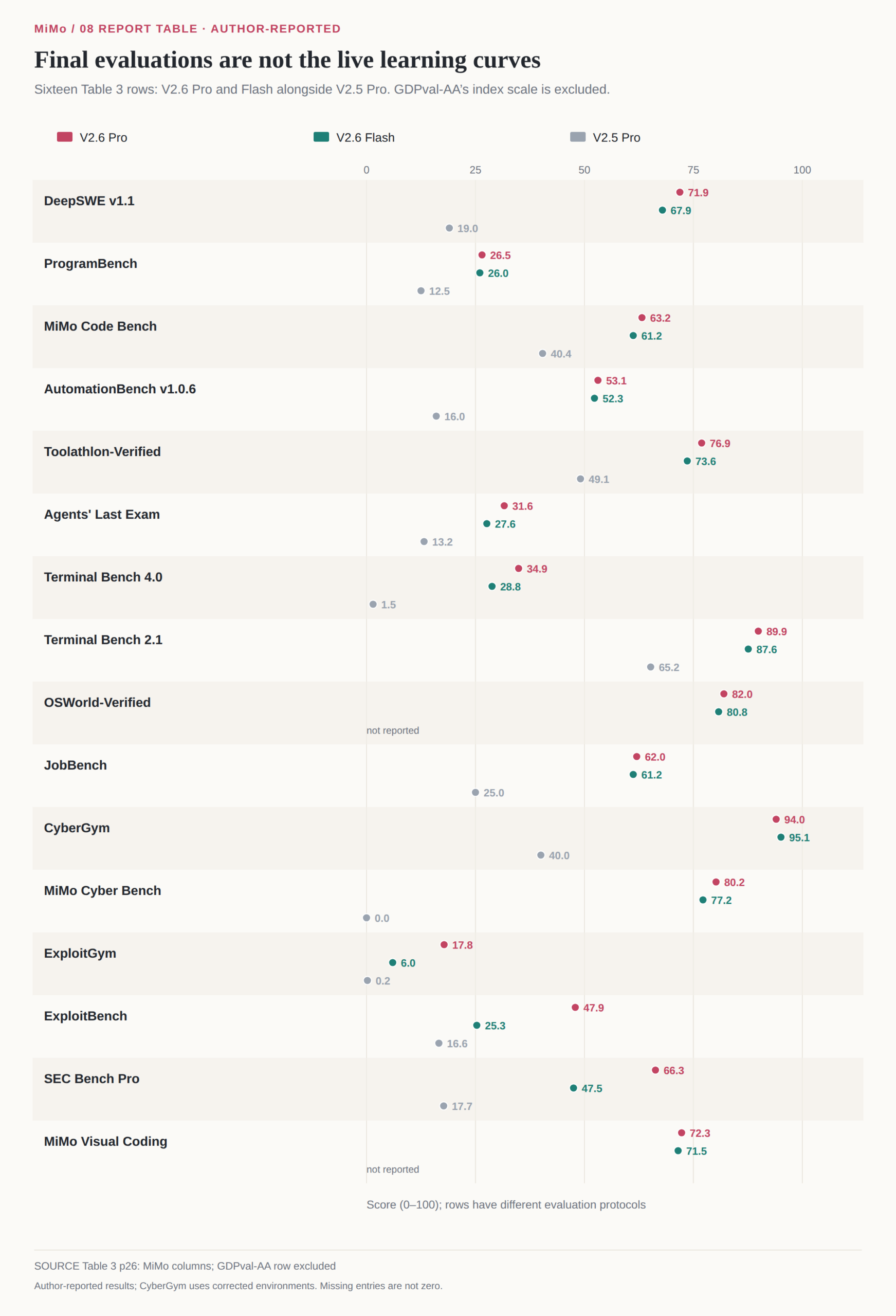
The report includes broader competitor comparisons, but those do not license merging different evaluation protocols into a universal ranking. GDPval-AA is an index rather than a percentage. CyberGym’s corrected environments deserve an explicit note. The announcement’s separate index and pricing claims are not needed to establish this article’s argument, so they are not used as substitutes for the report’s evidence.
The small model is a separate route through the ideas
The public 9B lane begins with Qwen3.5-9B and a distillation SFT dataset totaling 77.4 billion tokens, of which 27.2 billion bear loss. Input and observation tokens can be necessary context without being prediction targets. The loss-bearing subset should therefore not be added to the total as if it were a second dataset or a second compute bill. Report §7.1 and Table 4.
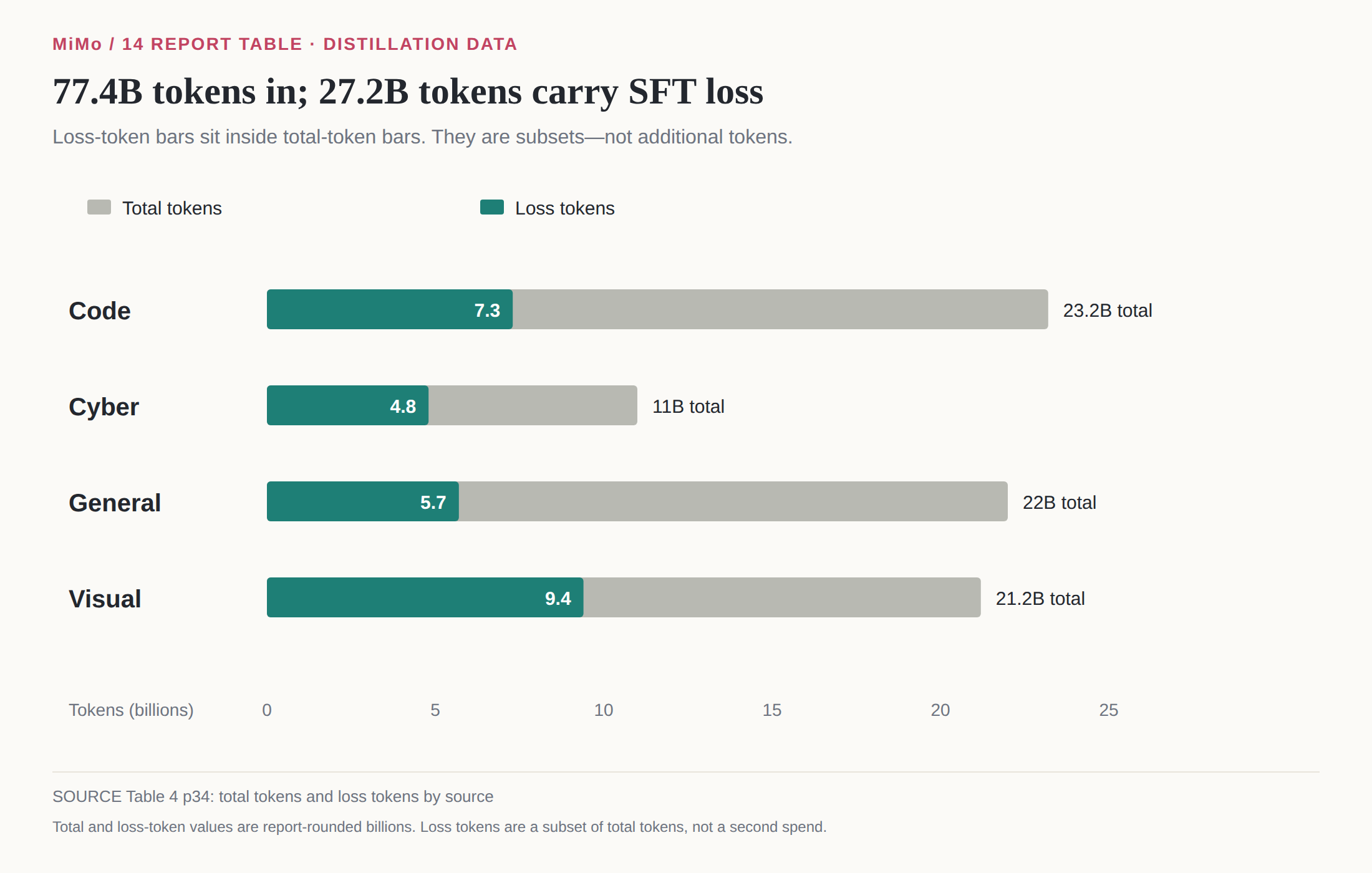
That distinction echoes the trajectory masks in RL. A training example can contain much more context than supervised action. Reading the total-token number as “the model was asked to predict every one of these tokens” would misdescribe the learning objective. Visual data has the largest reported loss-token count here without having the largest total-token count, illustrating why both measures deserve labels.
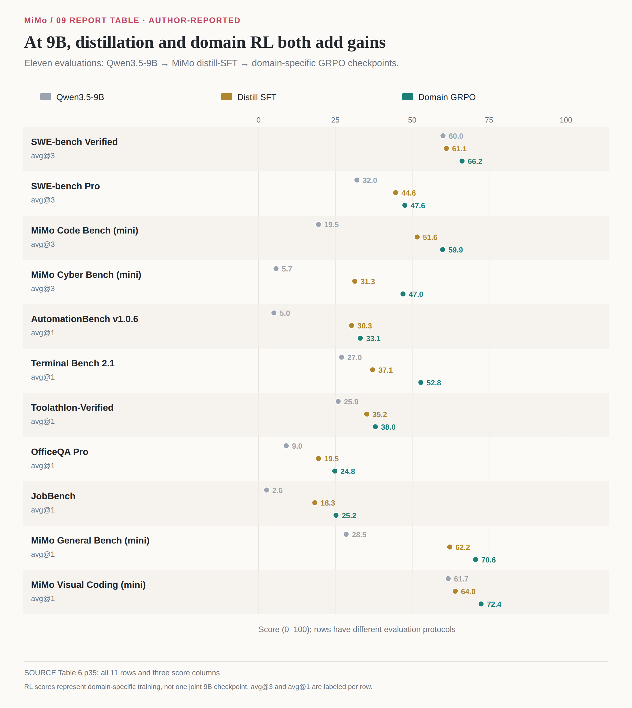
The released distilled checkpoint then seeds domain-specific GRPO experiments. Table 6 reports SWE-bench Verified rising from 61.1 after distillation SFT to 66.2 after domain RL; the mini cyber score rises from 31.3 to 47.0; Terminal Bench 2.1 rises from 37.1 to 52.8; the mini visual coding score rises from 64.0 to 72.4. These are different domain-trained checkpoints, not one joint 9B model simultaneously producing every endpoint.
The public lane also contains a separate multi-loop coding experiment. Four mini interaction systems are used in training: mini-mimocode, mini-bash, mini-claude-code and mini-codex. Evaluation then includes codex, claude code and mini-swe-agent as held-out interaction systems. The goal is to test whether improvement survives a change in the surrounding agent software rather than depending entirely on the exact training interface. Report Table 7.
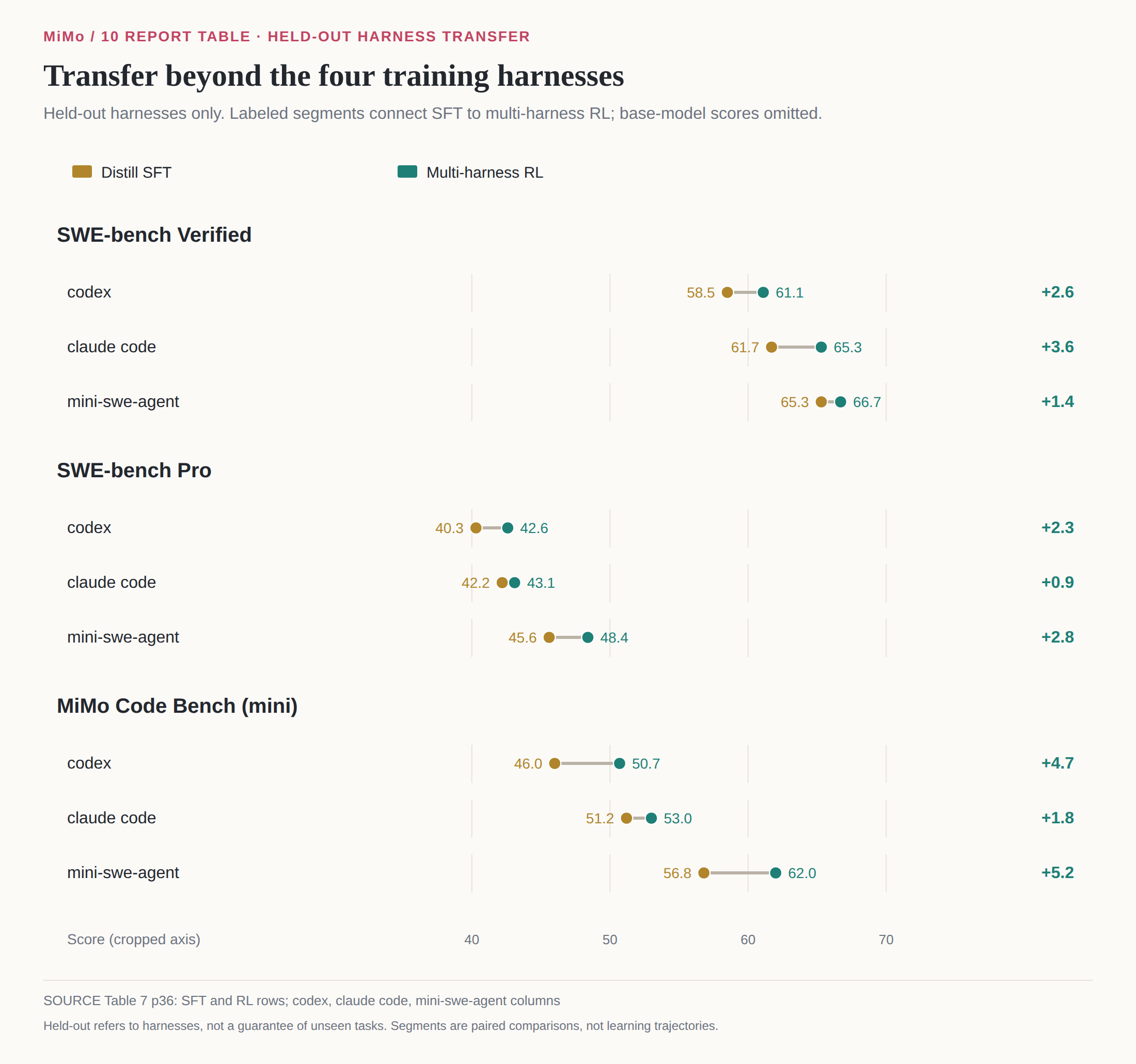
All nine displayed paired changes are positive. That is useful transfer evidence under the report’s setup, not proof of universal compatibility with arbitrary agent software. Versions, tool schemas, prompts and protocol adapters still matter. A model’s improved behavior has to survive the interface through which it acts.
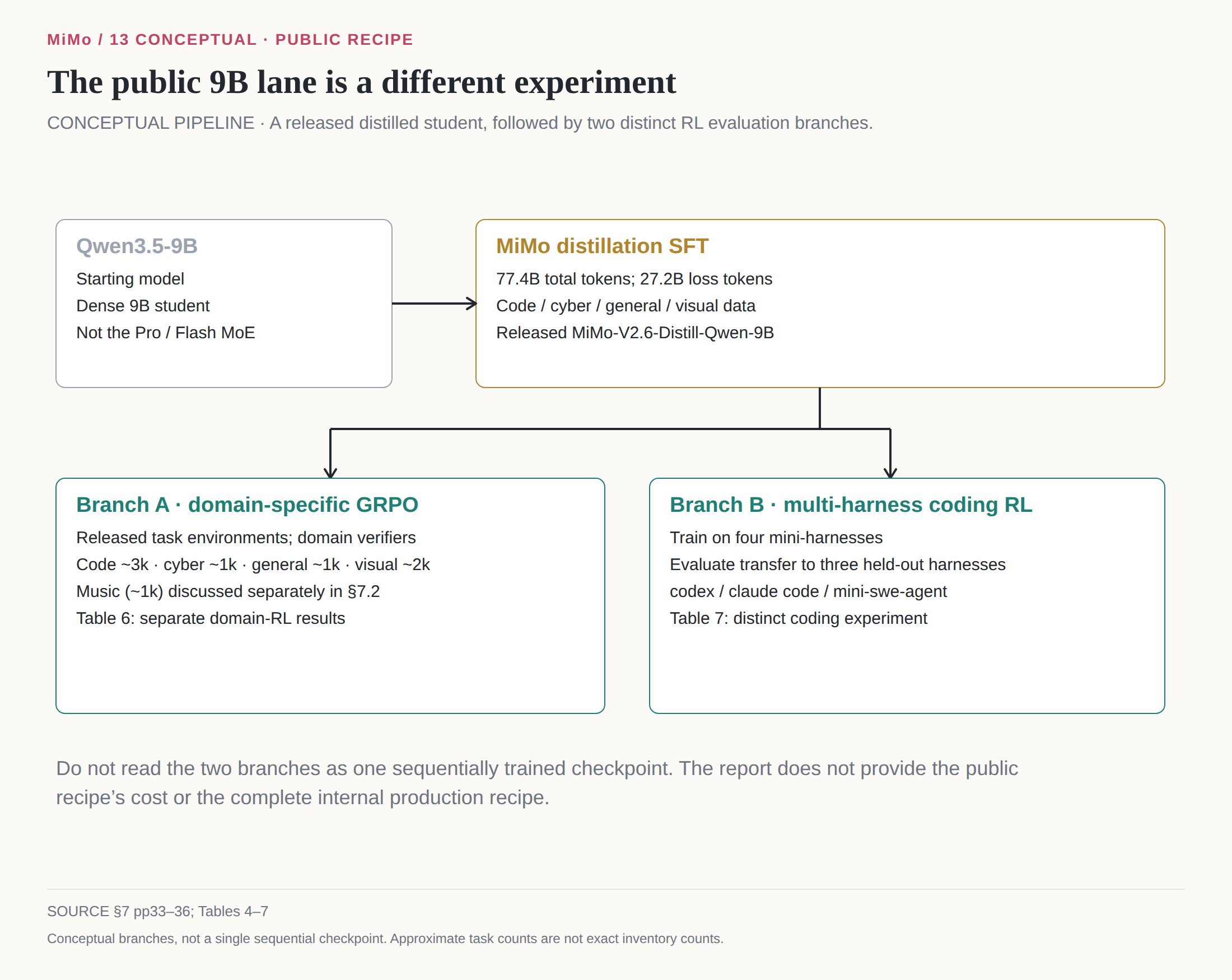
The branch diagram is the release in miniature: shared ideas, separate experiments, explicit boundaries. We can learn from the small route without pretending it recreates the large one. In fact, its smaller scope makes some of the interfaces easier to inspect, which is where the next set of lessons lives.
Three repositories meet at the trajectory boundary
The public software does not form one monolithic agent. The verl fork owns training, rollout integration, replay and optimization. mimoagent supplies agent, model, environment and dataset abstractions, together with mini implementations and adapters. uni-agent supplies the gateway and session machinery used by the Code route. Recipe code is the glue. Music takes a different route and uses neither agent submodule for its scoring loop. Public repository README; gateway adapter.
The source snapshots underlying this article are pinned: verl at a2ad9f6160b03ff2d47e59832bfb6b289f37c917, mimoagent at 467f0a19016f0ac4d63b8d17a1f0da9ba07f232c, and uni-agent at c63e0b01c375ebede95e01fe92bc367df24e5bf3. Pinning is not ceremony. Defaults, field names and a single condition around a mask can change the experiment. A link to a moving main branch would weaken claims about precisely what was inspected.
Code goes through a uni-agent rollout adapter, session gateway and mimoagent runner. The runner constructs the task environment, sets it up, creates the selected agent against a session endpoint, executes it, grades it and posts reward metadata. Cyber, General and Visual use direct recipe AgentLoop bridges with token tracing and environment actors. Music performs ordinary generation, extracts ABC text and runs a local conversion-and-scoring pipeline. Treating all five as the same gateway architecture would conceal real operational differences.
The gateway offers compatibility with several wire protocols, including OpenAI-style chat, Anthropic-style messages and OpenAI Responses, plus reward submission. Protocol compatibility is not simply renaming fields. Tool-call boundaries, thinking blocks, terminal markers and rollback semantics affect the transcript the trainer receives. Earlier adapter review found compatibility work around billing headers, unsupported redacted thinking and literal end-of-message markers in tool turns. Those are implementation-specific findings, not proof that every external client will work unmodified.
The session layer preserves generated token IDs and log probabilities rather than decoding an assistant response to text and re-tokenizing it later. Generated positions receive mask one; incremental observations receive mask zero. Requested log probabilities must match token counts. This keeps the training record close to the sampling record. Session implementation.
Prefix-chain selection handles histories that branch or roll back. It excludes reserved chains and mismatched tool schemas, ranks exact-prefix and rollback candidates, and declines ambiguous deepest rollback cases. Rolling back the last assistant response removes abandoned response IDs, masks, probabilities and policy-version marks, while retaining zero-length span records for alignment. This is the unphotogenic work required to make “the conversation” refer to the same sequence at every layer.
The public Code recipe selects the longest trajectory for export. The framework’s ability to represent multiple contexts therefore does not imply that the default recipe exports every context from every branch. Representation capacity and selection policy are separate choices. An article that says “multi-context support” without naming the selection setting can make the training data sound broader than it is. Code recipe; framework export path.
Rewards also have precedence. The framework prefers a reward posted by the runner, then a reward worker; without either it warns and leaves zero scores. It writes scalar reward at the final response position and stamps framework-controlled masks after merging extra fields. That order protects mask authority from arbitrary extras, but it does not make all reward failures semantically equivalent. A zero from a failed test and a zero from a missing grading path require different diagnosis.
Even completion has two meanings. The runner’s agent_completed flag records whether the agent reached Idle. It can still post finished=True for a successfully graded truncated run. The shipped Code configuration sets mask_unfinished_episode=false. So the attractive sentence “truncated rollouts are always masked” is wrong for this path. You have to inspect both the producer’s meaning and the consumer’s setting. Code runner; Code YAML.
The interface is sampled too
Code’s mixed selection uses a step-hash rule: seed, integer round and instance identity are joined with NUL separators, hashed, and mapped modulo the number of configured arms. The order of the arm specification therefore affects assignment. The seed is 20260911 in the outer launcher. Sibling rollouts for the same instance and round use the same selected arm. This provides a repeatable assignment rather than independently changing interfaces inside a prompt group. Code runner.
There is an optional group_advantage_by_harness setting, which can suffix group identities with agent type. It is false in both the inspected Code YAML and launcher. It should not be praised as a universally enabled safeguard for mixed-interface training. The default grouping story instead depends on the step-hash assignment keeping a group’s siblings on the same arm.
That difference is statistical, not cosmetic. If members of one group use very different tool affordances, raw reward differences may partly measure the interface rather than the policy’s choices. Grouping by interface can change the baseline, but it also changes group sizes and the amount of contrast available. The released default makes one choice; a modified experiment must reason through the consequences rather than merely enabling a reassuringly named switch.
There is a small source inconsistency worth retaining in a runbook. A docstring advertises a one-entry specification for a single-arm run, but the inspected parser rejects fewer than two entries. A reader copying the prose without checking the validator could begin debugging the wrong problem. We have not executed that path, so the careful conclusion is an identified code/documentation mismatch, not a tested workaround.
mini-codex introduces another boundary: programmatic tool calling. Its model-visible exec tool accepts raw JavaScript through a grammar-shaped interface; a wait tool handles yielded cells. The grammar accepts arbitrary source text. It is not a proof of valid or safe JavaScript. The documented execution environment is a fresh V8 isolate without direct Node, filesystem or network access, with persistence through store/load. Those properties are the external host’s contract, not independently verified security findings from this review. Code-mode wrapper.
Nested calls expose only configured tools and return through the agent’s execute_action path, preserving interceptors. Recursive exec/wait calls are rejected, and object versus freeform arguments are checked. This matters because programmatic composition must not become a side entrance around anti-hack or tool-validation logic. A loop written in JavaScript should still call the same guarded tool boundary as a direct model action.
The wrapper depends on an external codex-code-mode-host executable, pinned by the Python client to rust-v0.154.0. Resolution can use an explicit path, MIMOAGENT_CODE_MODE_HOST_PATH, or a cached/downloaded release asset; a mirror can be selected with MIMOAGENT_CODE_MODE_HOST_URL. Communication uses length-prefixed JSON over standard input/output, not newline-delimited JSON. Starting the arm may trigger a download unless the binary is staged. No binary was downloaded or executed here. Host discovery code.
Yielded, terminated, completed and failed cells remain distinct outcomes. The wrapper validates media encodings and result budgets and discards a failed host session on certain protocol errors. A JavaScript exception caught inside a cell is not the same event as an escaped transport or contract error. That separation helps preserve the meaning of failure, but actual host isolation, resource limits and teardown remain outside the completed audit.
The direct bridges keep a different kind of diary
Cyber, General and Visual each build an environment actor, bound setup with a timeout, obtain tools and template variables, create a model bridge, run the agent, request grading and construct an AgentLoopOutput. Cleanup is requested in a finally block, followed by actor termination. General supplies the final agent message to grading and adds MCP coordinates to the environment. Visual includes screenshot and group-grading metadata. Direct recipe sources.
The General TokenTrace stores the initial prompt once. New observations carry mask zero, generated tokens mask one, but both consume the response-region capacity. That last clause is easy to miss: a large tool response can exhaust the context budget without being a single loss-bearing action. A per-turn generation limit does not protect the whole episode from oversized observations. General token trace.
Finalization checks that response IDs, masks and log probabilities align, then clips them to the same response budget. Unlike the gateway’s strict probability-length requirement, this trace can pad a short supplied logprob list with zeros once logprobs are enabled. These are different contracts. One should not describe the direct bridge as if it were merely a thin wrapper around the gateway implementation.
Failure outputs also deserve literal reading. The bridges deliberately construct a minimal row with an EOS prompt token, an EOS response token, mask one and logprob zero rather than returning an empty tensor. The row preserves batch shape; it is not evidence that an actual policy sampled that token. Zero-gradient handling depends on later reward and infrastructure logic. General uses an invalid-reward sentinel, while ARVO and Webdev expose infrastructure flags. There is no single universal “every error is masked here” statement supported by the inspected paths.
The General environment documentation describes a two-container arrangement with system materials separated from the agent’s main container. That is a documented design intent. The entire construction, MCP and verifier implementation was not independently audited in the correction pass. A deployment needs the full task bundle: workspace, tools, state and verifier materials, not merely the General parquet. Static topology comments do not prove filesystem or network isolation under a real cluster configuration.
Finally is also not a magic word. Cleanup calls can fail, and the inspected bridges catch and log cleanup exceptions. Network partitions, forced termination and failed deletion can leave resources behind. The code requests cleanup; the source does not justify “pods never leak.” An actual deployment needs inventory reconciliation and a way to identify orphaned resources independent of the happy-path control flow.
What reaches the optimizer is a selected, rewritten record
The inspected V1 reward-to-advantage section has an order, and that order matters. It begins with optional KL reward shaping, then ARVO reference length shaping when enabled, then a Visual group-reward rewrite when its flag is present. Rollout correction follows. Optional infrastructure-UID exclusion precedes multi-trajectory GRPO. Optional deep-failure and marked-token edits follow advantages, then signed rebalance, ARVO tool penalties, metrics and the write of advantages and returns to TransferQueue. This describes the inspected section, not every earlier tensor transformation. Trainer shaping path.
Moving an operation across that boundary can change the objective. A length deduction before GRPO changes both an attempt’s score and the group baseline. A token edit after GRPO changes selected positions without rebuilding all scalar rewards. Filtering a group changes whether it enters training at all. These are different actions even when all three are casually called “penalties.”
For sessions with multiple outputs, only the final output by index participates in the scalar group-advantage computation. The resulting session advantage is broadcast back across that session’s outputs and multiplied by their response masks. This avoids treating every intermediate context as an independent success or failure, while still letting eligible generated tokens share the session outcome. Optional interface suffixes alter group identities, but, as noted, are not enabled by default in Code. Multi-output GRPO.
General’s invalid-reward sentinel has explicit handling in the GRPO kernel. Invalid scores are replaced with the mean of valid group scores, or zero if none exist, and invalid advantages are then explicitly zeroed. This is not the same as assuming that any isolated row has zero advantage. In the inspected singleton path, the baseline mean is set to zero and standard deviation to one; a nonzero singleton reward therefore remains nonzero. Public GRPO kernel.
The practical consequence is uncomfortable but necessary: changing an infrastructure reward convention can change gradients. A path that happens to be neutral with zero-valued error rewards may stop being neutral if errors receive another number. Likewise, the DAPO classifier checks a particular is_infra field. It does not infer infrastructure status from every nested error_category string or arbitrary sentinel. End-to-end metadata propagation remains a named coverage gap.
ARVO’s reference validator refuses incompatible deviations from its expected GRPO profile: no KL reward or loss, no standard-deviation normalization, DAPO filtering enabled and prompt-mean reduction, alongside its reference penalty settings. That is a recipe contract, not a claim that every domain must use those settings. Webdev, for example, disables DAPO group filtering in its YAML. ARVO validation; Webdev configuration.
The reference JSON is also not protected by an independent immutable numerical checksum in the inspected loader. The loader validates rule names and strategy, then treats loaded values as the reference against which overrides are compared. Editing the reference file changes that reference. This distinction matters for provenance: record the actual file or its digest with the run, not just the comforting phrase “reference config.”
The visual grader does not grade everything it sees
The public Visual reward is not the production coding GAR equation. It combines a group-relative aesthetic selection, a query-fit deduction and a runtime gate. The separation is deliberate: aesthetic preference should not masquerade as functional verification. Visual group driver; grader selection service.
The driver collects pending rows with existing screenshot paths and groups them by UID. The default minimum is four rows, with slices of eight, up to twenty-four concurrent group jobs, a 1,500-second overall wait budget and 1,200-second request timeout. Screenshot paths must be readable on the driver. If images exist only inside an inaccessible pod, this is not merely an artifact-management inconvenience; it changes which rows receive reward.
The service performs eight pick rounds. When group size matches the round count and is even, it uses Williams ordering; otherwise it uses randomized orderings. Multiple presentation orders try to reduce position effects in model judgments. At least five successful rounds are required for nonzero pick scores, and no-clear-difference or small-net-vote cases can zero the aesthetic component. The source comment’s claimed measured bias improvement was not independently reproduced here.
The pick prompt explicitly asks for clearly better and worse candidates rather than forcing a total ranking. Middling candidates may remain unranked. Functionality, correctness and requirement satisfaction are excluded from this aesthetic judgment. That is healthier than asking one vague “quality” score to carry every responsibility.
For a normal row, reward is (pick_norm − query_deduct + 2)/3, rounded to four decimal places. Query-fit scores at least 0.9, 0.6, 0.4 and 0.2 receive deductions of zero, 0.2, 0.4 and 0.8 respectively; below 0.2 the reward is zero. A runtime factor exactly equal to zero also floors reward. Missing runtime factor defaults permissively. Missing pick or query output is a missing result, not a valid zero score.
Invalid pending rows are replaced with the mean of valid pending judged rows for that UID before scalar reward is placed at the last generated token. A comment describes neutrality, but the substitution is only neutral if that mean equals the mean over the eventual whole GRPO group. Nonpending hard-zero rows can break that assumption. If no valid judged row exists, the driver leaves rows unchanged; too-small screenshot groups are skipped. These distinctions determine what the policy actually learns during partial grader failure.
Music has a compiler, not a listening panel
The public Music path asks the model for ABC notation. The scorer prefers a fenced ABC block containing an X: header, otherwise starts at the last such header. It runs abc2midi with a sixty-second subprocess timeout, extracts MIDI features and compares them with a reference baseline. Syntax and conversion gates can reject compiler errors, excessive bar warnings, blank-line formatting problems or conflicting channel programs. A missing executable raises a specific infrastructure error rather than silently assigning every sample a bad musical score. Music pipeline.
The feature model covers rhythm, texture, acoustics, tonality, register and structure, with weights 0.22, 0.20, 0.14, 0.16, 0.16 and 0.12. Features include note-length entropy, inter-onset intervals, density, polyphony, roughness, harmonicity, key certainty, in-scale pitches, range, voice leading, self-similarity and tension peaks. Band, low and high transforms compare these measurements with reference percentiles. Music score implementation.
A separate distribution term uses Jensen–Shannon divergence over pitch-class, interval and duration histograms. The combined score is 100 × (0.85 × base + 0.15 × dist_s), rounded to one decimal, then divided by one hundred and clipped into the unit interval by the pipeline. This is a transparent proxy: it rewards selected statistical properties and valid notation rather than pretending to hear music like a listener.
The limitation is equally concrete. The inspected compute_score path does not use ground_truth or extra_info to verify adherence to the musical request. A sample can score well on distributional musical features without satisfying a requested theme, instrumentation or structure. Feature extraction helpers and baseline-corpus provenance were not fully audited either. This does not make the recipe worthless; it tells us what experiment it is. It studies learning against a syntactic and feature-based proxy, not verified listener preference or audio fidelity.
Follow one group until the numbers stop being innocent
A small worked example helps connect the equations to the software. The numbers in this section are an illustration, not a sampled MiMo trajectory, a reported ablation or a measurement from the released recipe. Use four attempts rather than the production group of sixteen so the bookkeeping fits on the page.
Suppose their binary rewards are one, one, zero and zero. With a simple unnormalized mean baseline, the group mean is one half, so advantages are +0.5, +0.5, −0.5 and −0.5. Both passes initially receive the same positive signal. If the first pass used a broad patch that weakens a check while the second fixed the underlying bug precisely, the binary rewards do not encode that difference. The policy has no reason, from those four scalars alone, to prefer the second approach.
Now illustrate GAR with quality factors one half and one for the two passing attempts. Their original positive advantage sums to one. Their quality-weighted advantage sums to three quarters, so the compensating λ is four thirds. The revised positive advantages become one third and two thirds; the failures remain at minus one half each. The better pass receives more credit, the worse pass less, and the group still sums to zero in this uncapped example. No extra total positive advantage was created to achieve the preference.
This calculation exposes two dependencies. First, the quality judgment has to mean what we think it means. A grader fooled by verbosity can redistribute credit toward verbosity with perfect arithmetic. Second, the passing set must already exclude confirmed hacks. If the first “pass” came from reading a leaked answer, downweighting it as merely low quality is weaker than correcting its reward to zero and recomputing group statistics. Quality grading and integrity checking are connected but different jobs.
The length penalty introduces another dependency: ordering. Imagine a passing attempt whose length is one and a half times its successful-peer anchor, in a group whose pass fraction strictly exceeds the gate. Under the public ARVO reference ramp, with no deadzone, saturation at relative excess one, exponent 1.5 and maximum deduction 0.2, the deduction would be about 0.0707. This illustrates the public constants, not a production value. If a four-attempt group had exactly two passes and the gate were 0.5, the public rule would skip shaping because equality does not exceed the gate.
When that deduction occurs before group-relative advantages, it changes the baseline as well as the selected reward. A penalty on one passing row can therefore alter other rows’ relative advantages even if their own raw rewards are unchanged. That is not an accidental side effect; it follows from defining success comparatively. It is also why an implementation’s operation order belongs in the technical explanation rather than being dismissed as code organization.
Token-level signed redistribution asks a different question. For a separate illustration, imagine eight positive positions, each with advantage +0.5, of which two are flagged. The original positive mass is four. Flagged mass is one, clean mass three, so an unclamped α of four thirds moves the positive total onto the six clean positions. Flagged positions receive zero; clean positions together still sum to four. The policy is encouraged through different token decisions even though the scalar mass is unchanged.
For eight negative positions each at −0.5, again with two flagged, κ = 2 doubles the magnitude assigned to the flagged positions. Their negative magnitude becomes two. Choosing β = two thirds leaves magnitude two across the clean positions, retaining total negative magnitude four. The formula only works this way because β multiplies the clean term, not the entire negative branch.
Now change this illustrative κ to four while retaining a β floor of one half. Flagged negative magnitude becomes four and clean negative magnitude remains at least one and a half, for total magnitude five and a half rather than four. The floor binds, so exact conservation is impossible under those constraints. This is not a failed derivation or a reason to pretend the code ignored its own rule. It is the trade encoded by a minimum clean-token scale. Monitoring must report the resulting imbalance.
Return from arithmetic to the trajectory. The agent’s failed test command may produce thousands of observation tokens. Those tokens influenced what the agent did next but were not chosen by the policy. They should not receive the same loss mask as the command that caused the failure. If the observation is re-tokenized inconsistently, mask alignment can shift; if old policy probabilities are discarded, the importance correction loses its reference. A correct scalar reward cannot repair either problem downstream.
Then consider an infrastructure failure among the attempts. A missing grader result is not evidence that the attempt deserved the same reward as a failed solution. General’s explicit invalid-sentinel handling and Visual’s pending-row mean substitution take different approaches, with different conditions for neutrality. The simple four-number example does not justify replacing every missing value with zero or a group mean. Before doing so, ask which group the mean covers and which mask the next stage consumes.
Finally, suppose the group was dispatched too long ago. The replay buffer can discard it despite valid token alignment and a trustworthy reward. That discards expensive work, but respects an age budget intended to limit policy mismatch. Alternatively, a group may have no usable contrast and be filtered for that reason. Neither event is a low task score. They are selection decisions about whether the record is useful for this update.
By the time the optimizer sees its batch, the original interaction has passed through several kinds of judgment: task correctness, integrity, quality, efficiency, behavioral validity, infrastructure validity and temporal eligibility. Each has a different unit and a different failure mode. The final advantage tensor is small enough to move between processes; the chain of reasons that makes it legitimate is much larger. That chain is the training system this release lets us inspect.
Before a launch, read the parts that spend money
This runbook describes the inspected public entrypoints. It is not a transcript of a working installation. The default hardware shapes are launcher defaults, not measured minimum requirements, and reducing every number until it fits a small machine is not a validated adaptation. Tensor parallelism, context capacity and GRPO group contrast impose constraints that do not scale independently.
Start with an approved training environment and explicit permission for cluster access, downloads, package changes and paid judging. Keep task execution away from unrelated workloads and secrets. The agentic arms execute repository and tool commands inside environments whose setup and isolation need operational review. An OpenAI-compatible gateway is a protocol surface, not a reason to expose a service publicly. Authentication and firewall correctness were not audited here.
The expected dependency family includes CUDA, PyTorch, Megatron, mbridge, SGLang, FlashInfer, Ray and TransferQueue. The source selects these components; this review did not validate a complete tested dependency lock, driver matrix or memory capacity. There is deliberately no invented pip command that promises to assemble all of them correctly.
The checkpoint, tokenizer, chat template and task data must be visible where the workers use them, not just on the launch host. The public README names the distilled 9B model and RL dataset. Their presence in a catalog does not prove readiness on a cluster. The source layout also matters: the recipes expect submodule locations under third_party/mimoagent-osr and third_party/uni_agent. The research checkouts were sibling directories, which is sufficient for reading but not evidence that launcher imports resolve.
Code fixes the uni-agent root under the expected third_party location and permits MIMOAGENT_SRC to override the mimoagent source root. Verify the actual resolved imports before attributing a startup error to CUDA or the model. A source tree in the wrong place can fail long before any useful GPU work begins. Code inner launcher.
Code: inspect the resolved contract, not just the shell header
The launch chain is scripts/code/train.sh, then recipes/code/run_train.sh, then the verl main_ppo module. The outer script copies the default four-arm specification into a run-local directory and rewrites limits and timeouts there. That preserves the original configuration, but it means the copied specification is part of the experiment. Save it with the run.
The required inputs include MODEL_PATH, TRAIN_DATA and VAL_DATA. Training and validation paths below are deliberate placeholders, not an assertion that a validation parquet with that name is included in the release. Use a real, separately defined validation split, and document how it was obtained.
# Documentary example; execute only in an authorized, provisioned checkout.
export MODEL_PATH=/approved/checkpoints/MiMo-V2.6-Distill-Qwen-9B
export TRAIN_DATA=/approved/data/code-train.parquet
export VAL_DATA=/approved/data/code-validation.parquet
export KUBECONFIG=/approved/cluster/kubeconfig
export RUN_DIR=/approved/runs/code-run-001

PREFLIGHT_ONLY=1 bash scripts/code/train.sh
# Review resolved_config.yaml, run provenance and copied arm specifications.
# After a separate readiness decision:
bash scripts/code/train.sh
These commands are composed from inspected variable and entrypoint contracts. They were not run for this article. Code preflight performs a cluster precheck before configuration resolution; it is not a passive parser. “Preflight” names a launch mode, not a safety guarantee. Code launcher; Code inner launcher.
The outer Code defaults are TRAIN_BATCH_SIZE=64 and N=16, a nominal 1,024 rollouts before dynamic filtering. MAXLEN=262144 is the full context window; PROMPT_LENGTH=16384 is the prompt budget; HARNESS_TURN_MAX_TOKENS=32768 caps a model turn. These are three different bounds. Tool observations can occupy context without being generated output, and a long episode can contain many individually valid turns before exhausting its total window.
The default topology is eight nodes with eight GPUs per node, actor tensor parallelism eight and rollout tensor parallelism two. The outer launcher sets context parallelism to one even though the inner script has a default of two. Effective configuration, after outer values and overrides, is what matters. The capacity guard checks PPO_MAX_TOKEN_LEN_PER_GPU multiplied by ACTOR_CP against MAXLEN. Passing a shell variable through the wrong layer can leave a configuration that looks reasonable in isolation but fails the combined constraint.
Code sampling defaults to temperature 1.0, top-p 0.95 and top-k 20. LOSS_AGG_MODE is prompt-mean; standard-deviation normalization is false; both KL reward and KL loss are disabled. The presence of an unused coefficient field does not turn KL back on. The actor learning rate is 10⁻⁶ with weight decay 0.01. These values differ from production and should remain labeled as public Code defaults.
Concurrency has several scopes. GATEWAY_COUNT defaults to eight, MAX_CONCURRENT_SESSIONS to 2,048, and the server’s maximum requests is a separate setting of 128. A large session budget is not a claim that every session is simultaneously generating a token. Agent time includes tools, setup and grading. MODEL_REQUEST_TIMEOUT is 3,600 seconds with SDK retries set to zero in the copied specifications; AGENT_REQUEST_IDLE_TIMEOUT is 720 seconds; the trajectory timeout is 4,800 seconds. A timeout at one layer cannot be diagnosed reliably by looking at another layer’s budget.
Repetition detection is on by default, but repetition reward-zeroing and penalty are off. Tool-error and deep-failure penalties are also off. Detection, monitoring and intervention are distinct states. Enabling a monitor does not establish that its finding changes reward or stops the trajectory. The inner script also guards repetition early-stop against an inconsistent reward-zeroing setting. The MTP_ENABLE family is false by default and should not be renamed DFlash in a description of this recipe.
The run-local artifacts are the first things to preserve: resolved configuration, manifest, copied arm specifications, trajectory outputs, validation results and checkpoints. If a later edit changes an arm’s tool schema or timeout, a reproducibility record needs the effective copy, not just a Git commit that points to the original default.
The other four entrypoints are not aliases
Cyber uses scripts/arvo/arvo.sh. Its outer defaults retain 64 prompts and sixteen rollouts, a 262,144-token context, eight-by-eight GPU topology and actor/rollout tensor parallelism eight/two. Sampling uses top-p 1.0 and top-k −1, unlike Code. The trajectory budget is 28,800 seconds, setup timeout 900 seconds, and the stale threshold eight with drop strategy. Resume is disabled by default. Its reference penalty profile and strict validation deserve inspection before changing optimization settings.
General uses scripts/general/general.sh. Its defaults are 64 prompts and eight rollouts, a 262,144-token context with a 49,152-token prompt budget, four nodes of eight GPUs and actor/rollout tensor parallelism eight/four. The trajectory timeout is 1,200 seconds and setup timeout 3,600. Its trainer is synchronous even though rollout generation is marked asynchronous. A zero reward-timeout value has bridge-specific semantics; do not read it as an immediate timeout without tracing the consuming code.
General needs GA_TASK_ROOT and the complete environment bundle, plus GA_JUDGE_URL, GA_JUDGE_KEY and an explicitly chosen judge model/API. The outer script’s default model name is gpt-4o-mini. That is a source default, not a model called during this review. A later deployment should choose an approved endpoint intentionally rather than inheriting the name by accident. Its preflight branch resolves configuration to standard output rather than following the same mandatory manifest flow as the other inspected launchers. Remember that the configured General length penalty has no established consumer in the reviewed path.
Visual uses scripts/design/webdev.sh. Defaults are 32 prompts with eight rollouts, a 262,144-token context, eight-by-eight GPUs and actor/rollout tensor parallelism eight/four. Temperature is 0.6, top-p 0.95 and top-k 20. The trajectory timeout is zero, meaning unbounded at this layer rather than instantly expired; setup is bounded at 900 seconds and reward at 1,500. That combination makes external resource controls and clear failure monitoring more important, not less.
Visual also needs KUBECONFIG, POD_PROXY, DESIGN_GRADER_URL, judge credentials and a shared WEBDEV_DEBUG_DIR. Train and evaluation paths use different judge variables. Rendering services and browser dependencies require their own deployment review. Shared screenshot visibility is part of reward correctness, so test it across the actual writer and reader machines before interpreting missing judgments as model behavior.
Music uses scripts/design/music.sh. Its outer defaults are 32 prompts and eight rollouts, MAXLEN=116384, a 16,384-token prompt budget, eight-by-eight GPUs, actor/rollout tensor parallelism eight/four, 32 workers and sixteen reward workers. It is not pod-based agent interaction in the same sense as the other arms. The converter executable must exist on reward workers, not merely on the launch host.
Music is the clearest reason never to equate preflight with read-only. The inner script can run apt-get update/install before its preflight exit and can probe Ray workers by running the scorer. Approved preinstallation is preferable to discovering that fallback during a supposedly harmless check. The code-mode host in the mini-codex arm presents a different download hazard: starting it can retrieve an external executable unless one has been staged. Both behaviors were read, neither executed.
After prerequisites and explicit authorization, the documentary preflight forms are:
PREFLIGHT_ONLY=1 bash scripts/arvo/arvo.sh
PREFLIGHT_ONLY=1 bash scripts/general/general.sh
PREFLIGHT_ONLY=1 bash scripts/design/webdev.sh
PREFLIGHT_ONLY=1 bash scripts/design/music.sh
Choose the relevant domain; this is not an instruction to run all four in sequence. Omitting PREFLIGHT_ONLY after review selects the corresponding launch path. None of these examples substitutes for a separately approved smoke test. There is no universally safe tiny run obtained by lowering batch size, rollout count and GPU count at random. Public outer scripts; Music inner launcher.
Recovery begins before the crash
A good failure report asks which layer failed before assigning blame to the policy. Setup failure, tool failure, verifier failure, missing grader output, stale eviction and an actor-update OOM are not interchangeable events. They differ in whether useful work exists, whether a reward is valid and whether replay can preserve anything.
The public Kubernetes backend includes retries for pod creation and a structured exec-result contract. The earlier source review also found chunked upload handling for large payloads, hash verification and deletion on mismatch. Those are useful defensive mechanisms, not proof that the cluster cannot lose a pod or produce an ambiguous timeout. Preserve the returned reason as well as the exit code. Coercing every strange result into an ordinary nonzero process exit can erase the distinction between a command that failed and a command whose execution state is unknown. mimoagent environment implementations.
At the replay layer, inspect no-contrast filtering, missing configured metrics and stale drops. Missing metrics on a finished group can raise rather than silently inventing a value. Verify actual is_infra propagation. A sudden rise in zero rewards can indicate a policy regression, but it can also mean a judge endpoint moved, a test image failed, or error metadata stopped reaching the classifier.
For signed penalties, inspect before/after positive and negative mass and the scale-clamped indicators. A clamp is not necessarily a bug; it may be an intended safety limit, but it invalidates an unconditional conservation claim. If the modified run depends on exact sign-wise totals, its monitoring must show that the relevant denominators exist and caps did not bind.
Visual requires a different dashboard. Track rows judged and rewritten, too-small groups, short pick results, hook failures, infrastructure exclusion, dead non-infrastructure rows and actor gradient norm. The launcher explicitly warns that critic/score/mean can remain at a placeholder zero because the group rewrite happens in memory and may not be written back when KL reward shaping is off. A zero dashboard field can therefore disagree with the reward actually used for the update. Follow the field’s path before diagnosing collapse. Visual launcher monitoring notes; trainer shaping path.
Music needs a clean distinction between a low feature score and Abc2MidiMissing. The first is an outcome under the proxy. The second says the proxy could not be computed. Turning a missing binary into a normal bad score would train against an infrastructure condition the model cannot fix.
Checkpointing is similarly conditional. The inspected V1 save path writes actor state, optional critic state and dataloader data.pt. Asynchronous TransferQueue state is saved only if the installed TransferQueue supports checkpointing. The normal save writes a latest-iteration tracker; asynchronous actor checkpoint save skips that tracker write at this point. A directory’s existence is not enough evidence that every component completed. Checkpoint save/load path.
Load supports disabled, automatic and explicit resume-path modes. An explicit path must contain global_step_. Missing dataloader state produces a warning and restarts that component afresh. TransferQueue restoration is conditional. Pending or running prompts can be reissued from persisted prompt data, with stale trajectory keys cleared and dispatch age restamped. This is reissuing work, not resuming every pod and subprocess at the exact tool instruction where power disappeared.
Code defaults to disabled resume, and its launcher supplies a null resume path before forwarding trailing overrides. A documentary explicit recovery command is:
# Only after checkpoint completeness and deployment compatibility are checked.
bash scripts/code/train.sh \
  trainer.resume_mode=resume_path \
  trainer.resume_from_path=/approved/runs/code-run-001/checkpoints/global_step_5
Before using it, verify the checkpoint’s components, topology compatibility and installed queue support. The source review does not certify crash consistency, remote-storage atomicity or numerical continuity. Reissuing a prompt also does not clean up the old environment by itself; reconcile orphaned pods and artifacts separately. “Resume succeeded” should mean more than a process printed the next step number.
This is where the production failure account becomes useful without becoming a public recovery manual. Adjusting parallelism fixed one reported expert-imbalance OOM. It does not tell us exactly which parallelism setting should change in a new deployment. A CPU packing OOM suggests checking host-memory and payload pressure, not automatically reducing a model’s context limit before identifying the source. Failures provide diagnostic categories; they are not transferable commands without the surrounding state.
Keep these symbols on the same page
The report and code reuse letters and expose several different token budgets. A compact dictionary helps keep the mechanism legible without adding another table.
G and batch. G is rollouts per prompt. Production uses sixteen with 1,568 prompts per step. Public Code and Cyber also default to sixteen, but their prompt batches are 64; General uses eight rollouts with 64 prompts, while Visual and Music use eight with 32. These nominal products precede filtering. A prompt, a sequence and a sandbox are not interchangeable count units.
q, o, t and M. q is the task prompt; o is a sampled output sequence; t indexes positions; M selects loss-bearing positions. Observations can have mask zero and still occupy the context window. The public per-turn output cap, prompt budget and full MAXLEN therefore constrain different objects.
R and A. R is a reward; policy advantage A compares an attempt against its group. R_test gates the GRS product, while solution and behavior scores reduce a pass according to the rubric. General’s invalid-reward sentinel is explicitly handled by its kernel and should not be casually replaced by a different error value.
f and λ. In GAR, f is the quality factor for a passing attempt and λ is the common compensating multiplier. Uncapped redistribution preserves the summed passing advantage before subsequent centering. Caps and omitted quality-factor details limit exact reconstruction.
ℓ, X, δ, s, γ, B and the length gate A. ℓ is generated length; the reference ℓ* is a percentile of passing peers. X caps the reward deduction, δ gives tolerated excess, s marks saturation and γ shapes the ramp. B selects the percentile. This gate A is a pass-rate threshold, not policy advantage. Production constants remain unpublished; public ARVO constants are a separate reference profile.
h, κ, α and β. h flags behavior at a token or segment. κ strengthens flagged negative advantage, α compensates clean positives and β compensates clean negatives. Caps, floors and missing clean-token mass can prevent exact conservation. β does not scale the flagged negative term.
B_i, r_i, t_i, p_i and w_i. In the Sample Mixer, B_i is a retained-group target, r_i acceptance rate and t_i rollout duration. Demand m_i = B_i/r_i informs oversampling p_i and scheduling weight w_i. The mixer’s A_i is accepted count; its α blends target and deficit demand. Neither is the same object as its namesake in policy shaping.
W, TP, CP and EP. W is the production sliding-attention window, 128. Tensor parallelism splits tensor computation; context parallelism splits sequence work; expert parallelism distributes experts. They interact with memory and traffic in different ways. “More parallelism” is not a complete diagnosis or a complete fix.
Staleness and timeout. Production’s reported staleness is four. Public replay thresholds use prompt-dispatch age and vary by recipe. A trajectory timeout is wall-clock control, while per-step average staleness is a telemetry aggregate. Comparing them as if they had the same unit obscures the very failure one is trying to understand.
The boundary is part of the result
There is enough public material here to explain real mechanisms. There is not enough verified material to claim a full production reproduction. The distinction survives every stage of the article.
The source review independently covered all five outer launchers, several inner scripts and configurations, signed rebalance, General token tracing, Visual group reward, Music scoring and the mini-codex wrapper, plus selected trainer, replay, gateway, routing and checkpoint bodies. It did not read every engine kernel, every environment-construction method or the external V8 executable. Earlier verifier and adapter findings remain inherited from the companion implementation review rather than being presented as fresh exhaustive rereading.
The remaining gaps are substantive: General’s potentially unwired length shaping; uneven infrastructure metadata; conditional Visual missing-row neutrality; incomplete host isolation and renderer review; uninspected Music feature helpers and baseline provenance; dependency compatibility; image interiors; full task-bundle readiness; and complete checkpoint serialization behavior. No installed runtime was used to resolve those uncertainties. They constrain claims rather than becoming imaginary successful tests.
The production report also leaves out numerical settings for several penalties, grader-quality mappings and mixer bounds, along with detailed SFT information. The saved evidence does not contain numeric interiors for several ablation curves. The live API collection lost some optimization series. Missing observations remain missing in the figures. Those are limits of the evidence, not invitations to complete the picture by intuition.
What I take from MiMo-V2.6 is a demanding, practical standard for talking about agent training. Show the policy update, but also show how an observation becomes a masked token. Show a reward, but also the failure category that prevents a broken verifier from becoming a lesson. Show the benchmark gain, but identify the checkpoint, evaluation setting and interaction system that produced it. Show the launch script, but admit when no one in the review actually launched it.
The next agent does not become dependable because its training objective has an elegant name. It becomes more dependable, if the experiment works, because many small contracts hold at once: the task means what the verifier checks; the grader sees the artifact it claims to judge; the stored probability belongs to the sampled token; the replayed work is still eligible; the reward reaches the intended positions; the checkpoint preserves enough state to continue honestly.
Xiaomi has published a useful window into those contracts, along with smaller experiments that can be investigated in their own right. The bill and the restarts make the window better, not worse. They remind us that a training system is not a diagram with flawless arrows. It is a machine that spends real resources trying to keep its promises, and that the promises are the part worth learning to inspect.
Sources and figure provenance
The fourteen figures were drawn from saved evidence captured for this article on September 27, 2026. The live series endpoint returned HTTP 502 during the publication check, so its citations point to the public dashboard; the plotted values remain the saved observations, not a fresh fetch. Figures 1–6 use saved live API observations; Figure 7 combines live cost totals with report cost shares; Figures 8–11 and 14 use report tables or text-stated endpoints; Figures 12–13 are explanatory diagrams of documented structure. No plot contains invented curve interiors, inferred missing evaluations or synthetic uncertainty bands. Source links throughout the article pin the reviewed software snapshots. The charts distinguish reported experiments, saved telemetry and explanatory diagrams; none represents a training run performed for this article.